Pivot table - Formatting cells

[#1]

Hello,

In a pivot table, I would like to put the same background color for my dimensions: blue for product, green for company.

As you can see It doesn't work if the first cell is NULL in the table.

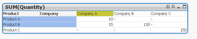
Do you know how I can have the format applied even if some values are NULL ?

Thanks for your answer

[enriquem]

Hello!

1.Select the properties in you Pivot Table

2.go to the Dimension tab

3.Select a color for each dimension that you select, like i show you. (you can do this to the expressions too)

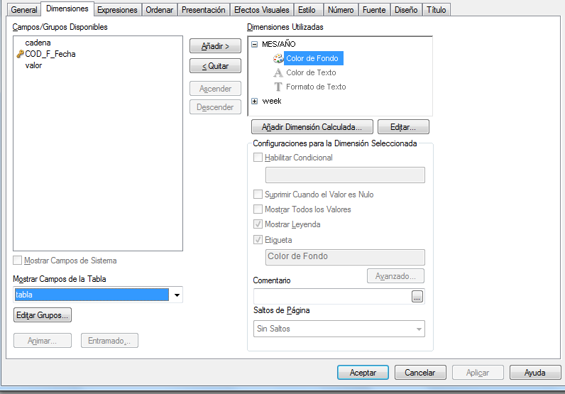
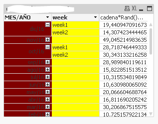
I put the red() color to the first, and yellow to the second.

4.Finally apply and accept. And your pivot table will look like this:

Regards

[#3]

Thanks for your answer.

It is exactly what I dit but it doesn't work in my example:

- one dimension in column, one dimension in row

- result of expression is null => Company b and Company c don't have any color because the first row (product a) is null

[el_aprendiz111]

Hi, 1 example

1

[#5]

I think I am not very clear with my request

I attached to this message my example where your solutions don't work.