Rank function

[#1]

Hello All,

I am running into an issue when using the Rank function.

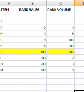
Requirement:  To design a chart that will show  ITEMS where Rank Sales and Rank Volume <=5.

Below image is the chart return from

DIMENTION: ITEM

TWO EXPRESSION :

          RANK (SUM (SALES))

          RANK(SUM(VOLUME))

Question : How do i eliminate , ITEM G highlighted in yellow from appearing on the chart.

Any suggestions will be appreciated.

Thank you.

Pranita

[#2 · Accepted solution]

Hello Shrestha,

Replace the item dimension with the following conditional dimension.

=if(aggr(RANK(SUM(VOLUME)),ITEM)<=5 or aggr(RANK(SUM(SALES)),ITEM)<=5,ITEM)

Then check supress if null for the conditional dimension.

Regards,

Kiran.

[#3]

Just the solution I was looking for.

Thank you Kiran !!

Regards,

Pranita