add rows in data sets

[priyarane]

Hi Community,

How to add rows in data set.

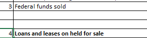
Currently we have data in Pivot table:

and we have to show like below:

it is one of the dimension for ex: Dim1 and Expr: Sum(Sales)

and we have to do in front end only, it is not possible to do in script part.

- Priya

[priyarane]

We are getting values from Dimension only, for Ex: Dim1

[settu_periasamy]

May be you can try with valuelist function (if you dimension values are less).

check the attached sample

[priyarane]

Hi Seetu, thanks for your efforts. Is there any way that we can avoid hard coding the values,like in dimension we have taken A, B C D so can't we avoid hard coding of this.

[settu_periasamy]

As i know, You can concat your dimension value and store it as a variable( this value should include single quotes and space character for displaying 2 empty rows - you can see that in my example )..

Use that variable in your valuelist.. then you can do the same in your expression too..

[priyarane]

Hi Ciaran,

as per you I have added it but I am getting out put like

But we need out put like

Dim

A

B

Dummy Row1

Dummy Row2

C

[priyarane]

Code

[varshavig12]

If your dimension consist of some limited no. of rows, then you can use pick-match.

[ciaran_mcgowan]

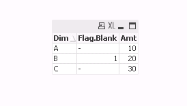
Hi Priya,

In your example, you are using the expression

if(Previous(RowNo())=2 OR Previous(Previous(RowNo()))=2, 1 ) AS Flag.Blank

You can't use RowNo() like this, it will always return the value of the row it's reading. You would need to use RowNo() when loading from your data source (in the original table),

Data:
LOAD RowNo() AS  Row,
    Dim,
    Amt
FROM

(ooxml, embedded labels, table is Sheet1);

Then use:

if(Previous(Row)=2 OR Previous(Previous(Row))=2, 1 ) AS Flag.Blank

Although, looking at this again, my other suggestion would serve your needs better. Simply load a Dummy table like this:

DummyData:
LOAD * Inline [
Dim
B1,
B2
];

This creates output of the following table:

Dim	Amt
A	10
B	20
B1	-
B2	-
C	30

Create a Straight Table with Dim & Amt as your Dimensions and this as your Expression:

if(Match(Dim, 'B1', 'B2'),'x',1)

Call the expression Flag and go to the Presentation tab and hide that column. In the Dimensions tab expand each dimension and insert the following code for the Text Color:

=if(Match(Dim, 'B1', 'B2'),White())

See my attached example.

[ciaran_mcgowan]

Hi Priya,

Did any of the suggestions here help you to solve your problem?