Unlock a world of possibilities! Login now and discover the exclusive benefits awaiting you.
- Qlik Community
- :
- All Forums
- :
- QlikView App Dev
- :
- help in
- Subscribe to RSS Feed
- Mark Topic as New
- Mark Topic as Read
- Float this Topic for Current User
- Bookmark
- Subscribe
- Mute
- Printer Friendly Page
- Mark as New
- Bookmark
- Subscribe
- Mute
- Subscribe to RSS Feed
- Permalink
- Report Inappropriate Content
help in
HI
i have a pivot table with dimension
i am attaching the sample app. please look into it and let me know the suggestions
- « Previous Replies
-
- 1
- 2
- Next Replies »
Accepted Solutions
- Mark as New
- Bookmark
- Subscribe
- Mute
- Subscribe to RSS Feed
- Permalink
- Report Inappropriate Content
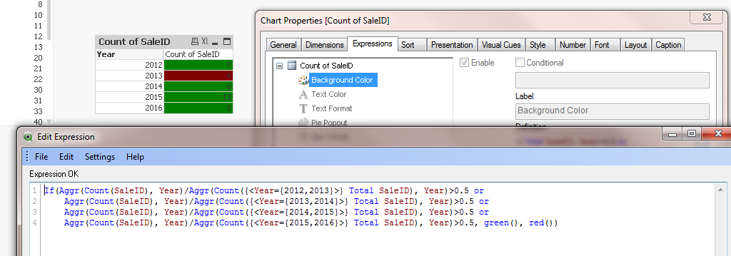
I came up with this atrocious expression, let me know if this works for you:
- Mark as New
- Bookmark
- Subscribe
- Mute
- Subscribe to RSS Feed
- Permalink
- Report Inappropriate Content
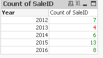
if you are looking for something like this, where the numbers are green or red
you want to expand the expression (the + sign) and go into Text Color and use the following expression
=if (Count(SaleID) > 5, rgb(0,130,0), RGB(255,0,0))
if you want the color of the cell to change to red or green, then isntead of putting the above expression in the txt color property place it in the background color property
- Mark as New
- Bookmark
- Subscribe
- Mute
- Subscribe to RSS Feed
- Permalink
- Report Inappropriate Content
Thanks Adam
I need to compare for every two years like 2012, 2013 ....... 2013 and 2014 ........ 2014 and 2015 like this
not for the whole years count of sales.
- Mark as New
- Bookmark
- Subscribe
- Mute
- Subscribe to RSS Feed
- Permalink
- Report Inappropriate Content
ahhh - sorry misunderstood
I think you want to use the same concept using set analyis in the expression of the color
- Mark as New
- Bookmark
- Subscribe
- Mute
- Subscribe to RSS Feed
- Permalink
- Report Inappropriate Content
Hi,
You can use the Above() function to get the value of the cell above, which will allow you to determine the text colour to apply. Something similar to this should work: if (above(Count(SaleID)) > Count(SaleID), red(), green());
- Mark as New
- Bookmark
- Subscribe
- Mute
- Subscribe to RSS Feed
- Permalink
- Report Inappropriate Content
thanks Adam for the response
i am trying it out but not success 
- Mark as New
- Bookmark
- Subscribe
- Mute
- Subscribe to RSS Feed
- Permalink
- Report Inappropriate Content
I came up with this atrocious expression, let me know if this works for you:
- Mark as New
- Bookmark
- Subscribe
- Mute
- Subscribe to RSS Feed
- Permalink
- Report Inappropriate Content
have you tried the expressions Sinan sent?
- Mark as New
- Bookmark
- Subscribe
- Mute
- Subscribe to RSS Feed
- Permalink
- Report Inappropriate Content
Hi Sinan,
Well if it works it's not wrong 
However, if there is a lot of data, that expression is going to run very slowly. Using the inter chart function Above() will allow you to get to the value in the cell above without having to do a whole load of recalculations.
George
- Mark as New
- Bookmark
- Subscribe
- Mute
- Subscribe to RSS Feed
- Permalink
- Report Inappropriate Content
Hello George
Thanks for the response but unfortunately above() is not near to the requirement,
- « Previous Replies
-
- 1
- 2
- Next Replies »