Unlock a world of possibilities! Login now and discover the exclusive benefits awaiting you.
- Qlik Community
- :
- All Forums
- :
- QlikView App Dev
- :
- Color shading in Pivot table
- Subscribe to RSS Feed
- Mark Topic as New
- Mark Topic as Read
- Float this Topic for Current User
- Bookmark
- Subscribe
- Mute
- Printer Friendly Page
- Mark as New
- Bookmark
- Subscribe
- Mute
- Subscribe to RSS Feed
- Permalink
- Report Inappropriate Content
Color shading in Pivot table
Hi,
How can I achieve the attached pivot table.
I want to shade the background color as blue and white as per the country and the product alternatively.
But it should be dynamic.
if product count is increasing at later point of time then the shading will also go with it.
Please help me out with the solution.
- « Previous Replies
-
- 1
- 2
- Next Replies »
Accepted Solutions
- Mark as New
- Bookmark
- Subscribe
- Mute
- Subscribe to RSS Feed
- Permalink
- Report Inappropriate Content
Hi Nikita,
You can see my screenshot below:
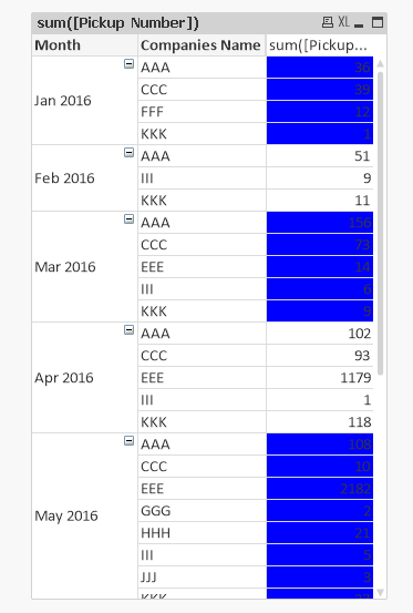
Hope this is what you want.
In my pivot table, you can see dimension are "Month" and "Companies name",
expression is sum([Pickup Number])
The color control is in
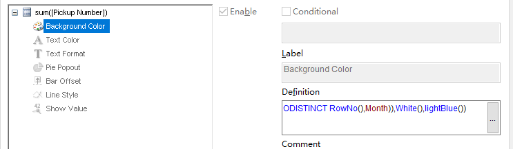
The definition is =if(Even(aggr(NODISTINCT RowNo(),Month)),White(),lightBlue())
The sort of Month is also very important in my solution.
Please try, any questions let me know.
Thanks.
Aiolos
- Mark as New
- Bookmark
- Subscribe
- Mute
- Subscribe to RSS Feed
- Permalink
- Report Inappropriate Content
May be use ARGB() instead RGB()
Using RGB() and ARGB() to define colors
- Mark as New
- Bookmark
- Subscribe
- Mute
- Subscribe to RSS Feed
- Permalink
- Report Inappropriate Content
Its not working.
Initially i was using the below expression
=IF(EVEN(SubField(RowNo(TOTAL)/8.1,'.',1)),RGB(179,234,255))
which is a hardcoded one because when my product list is increasing then the i have to modify expression again.
And if one country is having 7 products and another is having 8 products then also my expression is going wrong.
Later I have used the below expression but with this expression all country products and contract rate is going blue.
I want athe shading altrenatively
=if(count(DISTINCT([Product Type])),RGB(179,234,255))
- Mark as New
- Bookmark
- Subscribe
- Mute
- Subscribe to RSS Feed
- Permalink
- Report Inappropriate Content
Your last expression working? I don't think so..
May be try this way?
Color(FieldIndex('Product Type',Count([Product Type])))
Note - If not working, can you provide image?
- Mark as New
- Bookmark
- Subscribe
- Mute
- Subscribe to RSS Feed
- Permalink
- Report Inappropriate Content
Hi Nikita,
I found a way but it's a little complex, I think maybe there is better way to do this, I'm trying.
Now the method is :
You need to create another table and only have 2 columns. 1:Country 2. Rowno()
Then you use the field of rowno to change the background color. But your sort needs to be the same with the field.
Sample below.
Hope it's helpful.
Thanks.
Aiolos
- Mark as New
- Bookmark
- Subscribe
- Mute
- Subscribe to RSS Feed
- Permalink
- Report Inappropriate Content
Hi Aiolos,
I tried to open the QV file which you have attached here but it is not opening.
Can you please send me the expression.
Thanks.
- Mark as New
- Bookmark
- Subscribe
- Mute
- Subscribe to RSS Feed
- Permalink
- Report Inappropriate Content
Hi Nikita,
In my sample, in background color of expression, the expression is =if(Even(test),Green(),Blue())
test is another column
Thanks.
Aiolos
- Mark as New
- Bookmark
- Subscribe
- Mute
- Subscribe to RSS Feed
- Permalink
- Report Inappropriate Content
Hi Aiolos,
I am still not getting the desired result.All rows are getting blue colored.
Below is the expected result.
Desc: I have 2 dimension viz Country and Product.For 1 country I have 4 product while for other 4 or 5 or 2.
My color shading should happen accordingly and alternatively for country.
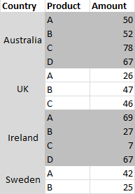
As of now I am using the below expression in my background
IF(EVEN(SubField(RowNo(TOTAL)/4.1,'.',1)),RGB(226,226,226))
Which is a hardcoded and working wrongly.
If I am using the above expression then for first country it is working fine but for others it is happening as below.
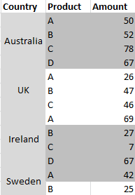
Please help me out with any generic solution.
Thanking you in advance.
Thanks,
Nikita
- Mark as New
- Bookmark
- Subscribe
- Mute
- Subscribe to RSS Feed
- Permalink
- Report Inappropriate Content
Hi Nikita,
You can see my screenshot below:
Hope this is what you want.
In my pivot table, you can see dimension are "Month" and "Companies name",
expression is sum([Pickup Number])
The color control is in
The definition is =if(Even(aggr(NODISTINCT RowNo(),Month)),White(),lightBlue())
The sort of Month is also very important in my solution.
Please try, any questions let me know.
Thanks.
Aiolos
- Mark as New
- Bookmark
- Subscribe
- Mute
- Subscribe to RSS Feed
- Permalink
- Report Inappropriate Content
Hello,
look here :
http://www.qlikfix.com/2010/11/25/custom-formatting-table-cells/
(I used the way via User Preferences (“Settings” -> “User Preferences”) and enabling the “Always Show Design Menu Items” option on the “Design”)
- « Previous Replies
-
- 1
- 2
- Next Replies »