Unlock a world of possibilities! Login now and discover the exclusive benefits awaiting you.
Announcements
Qlik and ServiceNow Partner to Bring Trusted Enterprise Context into AI-Powered Workflows. Learn More!
- Qlik Community
- :
- Forums
- :
- Analytics & AI
- :
- Products & Topics
- :
- App Development
- :
- Colour cell based on previous week numbers
Options
- Subscribe to RSS Feed
- Mark Topic as New
- Mark Topic as Read
- Float this Topic for Current User
- Bookmark
- Subscribe
- Mute
- Printer Friendly Page
Turn on suggestions
Auto-suggest helps you quickly narrow down your search results by suggesting possible matches as you type.
Showing results for
Contributor III
2019-11-21
10:40 AM
- Mark as New
- Bookmark
- Subscribe
- Mute
- Subscribe to RSS Feed
- Permalink
- Report Inappropriate Content
Colour cell based on previous week numbers
I have a pivot table like below with team down the left and Week number across the top and i want to be able to colour the cell based on if it is higher or lower than the previous week
is this possible in Qlik Sense?
| Week | ||||
| Team | 1 | 2 | 3 | 4 |
| A | 27 | 10 | 56 | 72 |
| B | 1 | 69 | 20 | 72 |
| C | 0 | 91 | 17 | 25 |
| D | 33 | 84 | 63 | 66 |
| E | 25 | 86 | 61 | 57 |
507 Views
2 Replies
Creator III
2019-11-21
01:22 PM
- Mark as New
- Bookmark
- Subscribe
- Mute
- Subscribe to RSS Feed
- Permalink
- Report Inappropriate Content
Load Script:
Data:
load * inline [
Team, Week, Value
A,1,27
A,2,10
B,1,1
B,2,69
];
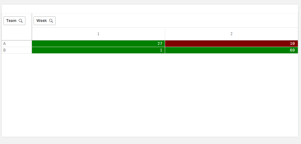
Color expression:
if(sum(Value) - before(sum(Value)) < 0 , red(),green())
Result:
490 Views
Contributor III
2019-11-22
02:45 AM
Author
- Mark as New
- Bookmark
- Subscribe
- Mute
- Subscribe to RSS Feed
- Permalink
- Report Inappropriate Content
great thanks so if my fields are as below what do i need to put in the script?:
Team = SUPPLIER_SUMMARY
Week = WEEKENDING_DATE
Value = Count(NOTICE_NUMBER)
473 Views
