Unlock a world of possibilities! Login now and discover the exclusive benefits awaiting you.
- Qlik Community
- :
- Forums
- :
- Analytics & AI
- :
- Products & Topics
- :
- App Development
- :
- Re: How to add conditional formatting in a pivot t...
- Subscribe to RSS Feed
- Mark Topic as New
- Mark Topic as Read
- Float this Topic for Current User
- Bookmark
- Subscribe
- Mute
- Printer Friendly Page
- Mark as New
- Bookmark
- Subscribe
- Mute
- Subscribe to RSS Feed
- Permalink
- Report Inappropriate Content
How to add conditional formatting in a pivot table
Hi I would like to add conditional formatting in a pivottable. I would like to be every value under 70% to be red, between 70 and 85 to be orange and above 85 to be green.
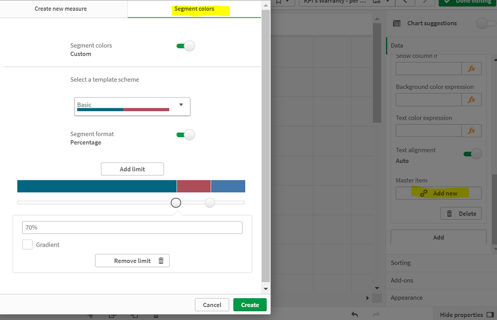
I know I should use master items under measures though when I fill in the specifics under segment colors and then create, nothing happens to my table. The colors remain white. Also I would like to have different colors then displayed in the image -> how to adjust?
- Mark as New
- Bookmark
- Subscribe
- Mute
- Subscribe to RSS Feed
- Permalink
- Report Inappropriate Content
hi,
find the link
https://community.qlik.com/t5/New-to-QlikView/Change-color-in-a-pivot-table/m-p/263423
ksrinivasan
- Mark as New
- Bookmark
- Subscribe
- Mute
- Subscribe to RSS Feed
- Permalink
- Report Inappropriate Content
You can create conditions background and text color like in Pivot table
If([Your measure]<=Num(0.7, '#,0%'), Red(), If([Your measure]>Num(0.7, '#,0%') and [Your measure]<=Num(0.85, '#,0%'), Yellow(), Green()))
- Mark as New
- Bookmark
- Subscribe
- Mute
- Subscribe to RSS Feed
- Permalink
- Report Inappropriate Content
Hi,
In Pivot table, under the expression, if you expand the expression further down there is the section for background and text colour expression. In there you can define the criteria you wanted to use for conditional colour changes.
- Mark as New
- Bookmark
- Subscribe
- Mute
- Subscribe to RSS Feed
- Permalink
- Report Inappropriate Content
You should be able to add under background expression for the Measures.
If([measure]<=Num(0.7, '#,0%'), Red(), If([measure]>Num(0.7, '#,0%') and [measure]<=Num(0.85, '#,0%'), Yellow(), Green()))
Also if you would like to have a specific shade of color, you can use hex code as well.

