Unlock a world of possibilities! Login now and discover the exclusive benefits awaiting you.
- Qlik Community
- :
- Forums
- :
- Analytics & AI
- :
- Products & Topics
- :
- App Development
- :
- Re: Qlik sense background color expression - Condi...
- Subscribe to RSS Feed
- Mark Topic as New
- Mark Topic as Read
- Float this Topic for Current User
- Bookmark
- Subscribe
- Mute
- Printer Friendly Page
- Mark as New
- Bookmark
- Subscribe
- Mute
- Subscribe to RSS Feed
- Permalink
- Report Inappropriate Content
Qlik sense background color expression - Conditional Formatting
Hi,
How can I make a conditional formatting in a Pivot Table?
I mean, I want to make background RED If the value is less than 0.
What formula should I write the background color expression?
Please find attached.
Thanks in advance.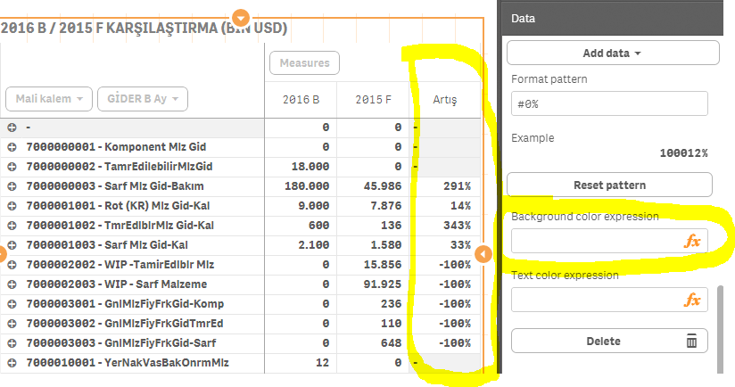
- Tags:
- gysbert wassenaar
Accepted Solutions
- Mark as New
- Bookmark
- Subscribe
- Mute
- Subscribe to RSS Feed
- Permalink
- Report Inappropriate Content
Hi Fatih,
You should try the following expression:
=if(Artis>0.5,red(),blue())
or
=if(Artis>0.5,rgb(123,12,125),rgb(255,255,255)
HTH
G.
- Mark as New
- Bookmark
- Subscribe
- Mute
- Subscribe to RSS Feed
- Permalink
- Report Inappropriate Content
Hi Fatih,
You should try the following expression:
=if(Artis>0.5,red(),blue())
or
=if(Artis>0.5,rgb(123,12,125),rgb(255,255,255)
HTH
G.
- Mark as New
- Bookmark
- Subscribe
- Mute
- Subscribe to RSS Feed
- Permalink
- Report Inappropriate Content
Hi Fatih,
You can use the expression which under grinder provided an will work perfectly. If you have any complex colour expressions you can even make use of ColorMix() function to achieve it.
Thanks,
Sangram Reddy.
- Mark as New
- Bookmark
- Subscribe
- Mute
- Subscribe to RSS Feed
- Permalink
- Report Inappropriate Content
Thank you for your answer undergrinder
- Mark as New
- Bookmark
- Subscribe
- Mute
- Subscribe to RSS Feed
- Permalink
- Report Inappropriate Content
Hi,
As sangram suggested, you can use colormix1 or colormix2 for gradient coloring. Eg: =ColorMix1(Count(distinct [columnA])/Count(columnB),white(),green())