Associate chart problem

[#1]

Hi,

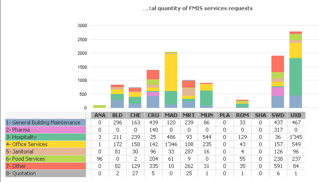
I actually have this chart

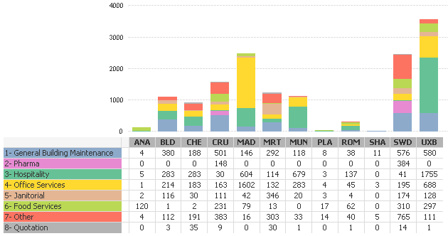
It represent the number of service request by Site.

I have 2 different chart, one pivot table and a combine bar chart.

My problem is that I have a calendar based on request date, and somes Site wasn't exist in 2014 for example so if I select 2014 my bar chart is not align with my pivot table and I dont know how to handle this.

I want to always display every Site on my pivot table like i did in my bar chart...

Ex 2014 --> PLA and SHA desappear

Thanks for your help

[erjohnso]

Change your expression in the pivot to:

=count(ITEMID)+sum({1} 0)

This way, all dimensions will always return at least a 0 no matter what criteria is selected.

[#3]

Hi,

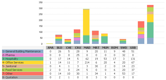
Hum, think i miss something else! The problem is in the last screenshot: "Supress Zero Values"

If I check it, i have this:

And if I uncheck It works BUT I have a null row like:

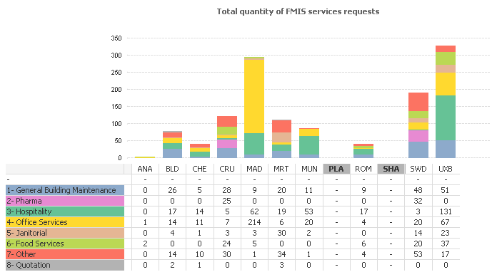
Without this first row it will be perfect..

[#4]

Hi, it works, yes, can you explain why?

But I have another problem, the backgrond color of my "vigs category" dimension desapear if i select for example 2014... Do you know why?

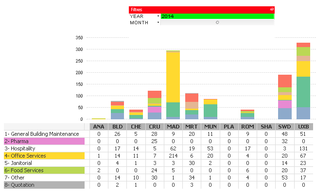
Thanks a lot.

[sunny_talwar · Accepted solution]

Try this as your background color expression:

=if(Only({1} [VIGS CATEGORY]) = '3- Hospitality',rgb(102,194,150),

if(Only({1} [VIGS CATEGORY])='1- General Building Maintenance',rgb(141,170,203),

if(Only({1} [VIGS CATEGORY])='4- Office Services',rgb(255,217,47),

if(Only({1} [VIGS CATEGORY])='7- Other', rgb(252,115,98),

if(Only({1} [VIGS CATEGORY]) = '6- Food Services', rgb(187,216,84),

if(Only({1} [VIGS CATEGORY]) = '2- Pharma', rgb(231,138,210),

if(Only({1} [VIGS CATEGORY])='5- Janitorial', rgb(229,182,148),

if(Only({1} [VIGS CATEGORY]) = '8- Quotation', rgb(179,179,179)))))))))

[erjohnso]

It works because we are calculating an expression for every dimension no matter what time period is selected.

The formatting for the color codes would need to be updated to include the {1} set identifier as well.

[#7]

Thanks to Both of you Eric and Sunny, it works very well now! 😃