Conditional Formatting on a Pivot Table

[#1]

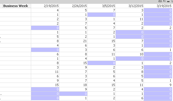
I attached a qvw where i created a pivot table showing the count of sales per employee for each business week.

I want to color code the people to tell me who hasn't sold anything in 1 week, 2 weeks , 3 + weeks and then someone who has null/zeros for all weeks shown (never sold anything).  I need the conditional formula for the background to calculate from the most current week in the data.

I don't care about which rgb codes at this time that are used.

Any suggestions are greatly appreciated.

Thanks,

Robyn

[a_mullick]

Hi Robyn,

You've probably thought of this already, but I think the easier solution is test the value of the expression cell. If it's zero, then colour the background. I can't find a way to conditionally highlight the dimension (based on an expression) so would be interested to hear of a solution.

Thanks,

Azam

[stigchel]

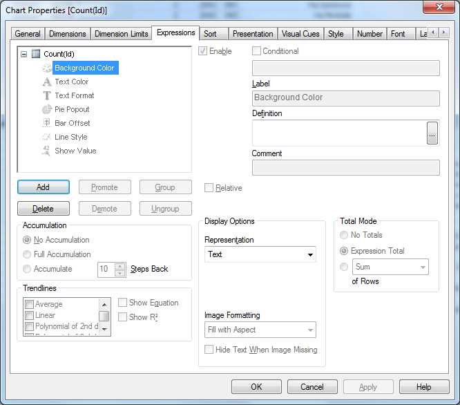
For the Dimension AND Expression click on the + sign, it will expand and there is a background color option, you can use the following expression

=if(Column(1)=0,rgb(200,0,0))