Unlock a world of possibilities! Login now and discover the exclusive benefits awaiting you.
- Qlik Community
- :
- All Forums
- :
- QlikView App Dev
- :
- Re: Count in Pivottabelle bzgl. Farbauswahl
- Subscribe to RSS Feed
- Mark Topic as New
- Mark Topic as Read
- Float this Topic for Current User
- Bookmark
- Subscribe
- Mute
- Printer Friendly Page
- Mark as New
- Bookmark
- Subscribe
- Mute
- Subscribe to RSS Feed
- Permalink
- Report Inappropriate Content
Count in Pivottabelle bzgl. Farbauswahl
Hallo zusammen,
ich habe eine Pivottabelle gebaut in der ich Farben einbauen muss. Wenn in einer Spalte 1x das Word 'Da' vorkommt soll dieses grün sein. Sobald das Wort 'Da' 2x vorkommt sollen diesen beiden Felder rot sein.
Bisher habe ich folgendes implemeniert was allerdings nicht funktioniert!
=if(count(Info = 'Da') >= 2, red()))
Was müsste ich anpassen?
Viele Grüße
- Mark as New
- Bookmark
- Subscribe
- Mute
- Subscribe to RSS Feed
- Permalink
- Report Inappropriate Content
May be this:
=If(Count({<Info = {'Da'}>} Info) >= 2, Red())
or
=If(Count(If(WildMatch(Info, '*Da*'), Info) >= 2, Red())
Best,
Sunny
- Mark as New
- Bookmark
- Subscribe
- Mute
- Subscribe to RSS Feed
- Permalink
- Report Inappropriate Content
Hi Thomas
you can use function SubStringCount
if(SubStringCount(Columnname,'Da')>1,red(),Green())
Hope this solves your problem else just share sample app
regards,
Bhagirath
Mark answer Correct/helpful
- Mark as New
- Bookmark
- Subscribe
- Mute
- Subscribe to RSS Feed
- Permalink
- Report Inappropriate Content
This solution doesn´t work. Look at my picture there ... for the 3 line the 2 'Da' must be colered in red!
Thank you
- Mark as New
- Bookmark
- Subscribe
- Mute
- Subscribe to RSS Feed
- Permalink
- Report Inappropriate Content
This solution doesn´t work. Look at my picture there ... for the 3 line the 2 'Da' must be colered in red!
Thank you
- Mark as New
- Bookmark
- Subscribe
- Mute
- Subscribe to RSS Feed
- Permalink
- Report Inappropriate Content
Would you be able to post a sample application??
Best,
Sunny
- Mark as New
- Bookmark
- Subscribe
- Mute
- Subscribe to RSS Feed
- Permalink
- Report Inappropriate Content
if(SubStringCount(Columnname,'Da')>1,red(),Green())
- Mark as New
- Bookmark
- Subscribe
- Mute
- Subscribe to RSS Feed
- Permalink
- Report Inappropriate Content
...
- Mark as New
- Bookmark
- Subscribe
- Mute
- Subscribe to RSS Feed
- Permalink
- Report Inappropriate Content
Do you want the count across your Werk dimension or AutoNr Dimension?
Best,
Sunny
- Mark as New
- Bookmark
- Subscribe
- Mute
- Subscribe to RSS Feed
- Permalink
- Report Inappropriate Content
Is this how you want it? 1st chart is count by the dimension Werk and second is by AutoNr
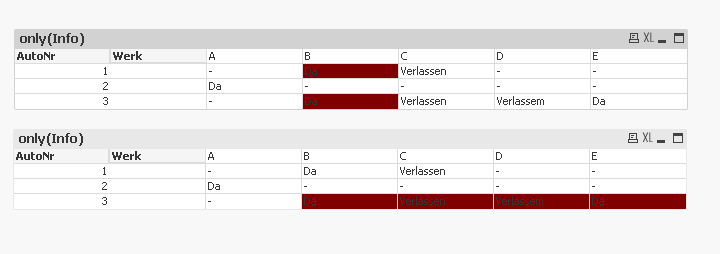
Color expression for the first chart: =If(Aggr(NODISTINCT Count({<Info = {'Da'}>} Info), Werk) >= 2, Red())
Color expression for the second chart: =If(Aggr(NODISTINCT Count({<Info = {'Da'}>} Info), AutoNr) >= 2, Red())
Attaching the application also.
Best,
Sunny