Unlock a world of possibilities! Login now and discover the exclusive benefits awaiting you.
- Qlik Community
- :
- All Forums
- :
- QlikView App Dev
- :
- Re: Help required to create complicated chart
- Subscribe to RSS Feed
- Mark Topic as New
- Mark Topic as Read
- Float this Topic for Current User
- Bookmark
- Subscribe
- Mute
- Printer Friendly Page
- Mark as New
- Bookmark
- Subscribe
- Mute
- Subscribe to RSS Feed
- Permalink
- Report Inappropriate Content
Help required to create complicated chart
I want to create a chart something like below one. The values that you see is the count of TRUE value against the each city for the selected date range(Based on the date range you have more number of month columns dynamically). It should count the number against each city based on the below expressions.
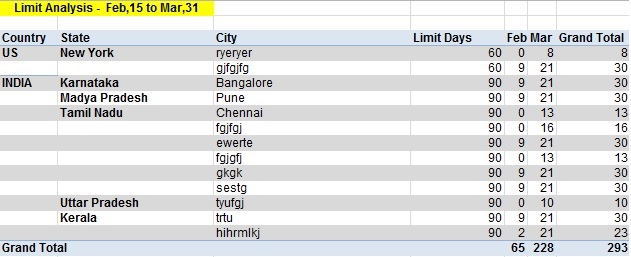
IF(
IF(Limit_Days='l_30',[30 days],
IF(Limit_Days='l_60',[60 days],
IF(Limit_Days='l_90',[90 days],
IF(Limit_Days='TBD',[60 days)
)
)
)<1
,sum(TOTAL{<Period = {'>$(=date($(VMaxPeriod)-$(VDays))) <=$(=date($(VMaxPeriod))) '}>} 1),
sum(TOTAL{<Period = {'>$(=date($(VMaxPeriod)-$(VDays))) <=$(=date($(VMaxPeriod))) '}>} 0))
Has anyone created a similar chart like this? Can you please help on the same since it doesn't looks to be straight forward.
- Tags:
- pivot table format
- « Previous Replies
-
- 1
- 2
- Next Replies »
- Mark as New
- Bookmark
- Subscribe
- Mute
- Subscribe to RSS Feed
- Permalink
- Report Inappropriate Content
Any help from any one about creating the above chart?
- Mark as New
- Bookmark
- Subscribe
- Mute
- Subscribe to RSS Feed
- Permalink
- Report Inappropriate Content
Hi,
Do you want to create the chart like your screenshot?
Hope you have Month Field. So, you can create the Pivot table, Include the Month Field in your dimension.
Try with your expression (believe it is working)
can you create the sample with dummy data? it would be helps us to resolve your question.
- Mark as New
- Bookmark
- Subscribe
- Mute
- Subscribe to RSS Feed
- Permalink
- Report Inappropriate Content
Yes I want to create a chart similar to one mentioned in the screen shot. We dont have Month field in our DM.We are just creating it using MonthName(Period) for Month Field and dragging it to the top of expression to make it as cross tab. Basically what i want(Under the month) is that count of number of days the value is < 1 in a month(Basically count of TRUE value of a month based on the below expression).
Please let me know if the requirement is not clear yet.
=IF(
IF(maxstring({<$(e_DateRange)>}Limit_Days)='last_30',$(e_Days('l_30')),
IF(maxstring({<$(e_DateRange)>}Limit_Days)='last_60',$(e_Days('l_60')),
IF(maxstring({<$(e_DateRange)>}Limit_Days)='last_90',$(e_Days('l_90')),
IF(maxstring({<$(e_DateRange)>}Limit_Days)='TBD',$(e_Days('l_60')))
)
)
)<1
,replace(sum(TOTAL{<Period = {'>$(=date($(VMaxPeriod)-$(VDays))) <=$(=date($(VMaxPeriod))) '}>} 1),1,'TRUE'),
replace(sum(TOTAL{<Period = {'>$(=date($(VMaxPeriod)-$(VDays))) <=$(=date($(VMaxPeriod))) '}>} 0),0,'FALSE')
)
- Mark as New
- Bookmark
- Subscribe
- Mute
- Subscribe to RSS Feed
- Permalink
- Report Inappropriate Content
So, you are using Calculating Dimension. what you are getting now, if you are using the above mentioned Expressions?
Can you post the screen shot?
Try to look on the Pick Match function also..
- Mark as New
- Bookmark
- Subscribe
- Mute
- Subscribe to RSS Feed
- Permalink
- Report Inappropriate Content
Yes we are using the calculated dimension. I am getting 1 and 1 respectively in both the months. Sorry not possible to attach the screen shot now as it has real data and what i mentioned above is just for your understanding.
By the way not able understand how i will make use of Pick and Match function? Could you please explain
- Mark as New
- Bookmark
- Subscribe
- Mute
- Subscribe to RSS Feed
- Permalink
- Report Inappropriate Content
i'm not able to assume what's happened. Someone will help.
- Mark as New
- Bookmark
- Subscribe
- Mute
- Subscribe to RSS Feed
- Permalink
- Report Inappropriate Content
Ok I know it is very difficult to work without any sample data. I wish to attach but due to security reason I am not attaching any.
- Mark as New
- Bookmark
- Subscribe
- Mute
- Subscribe to RSS Feed
- Permalink
- Report Inappropriate Content
Just to wanted to know how to take the count of TRUE values show the same against month after doing cross tab. That would be much helpful.
- Mark as New
- Bookmark
- Subscribe
- Mute
- Subscribe to RSS Feed
- Permalink
- Report Inappropriate Content
Hi All,
Basically I want to count only those days where the values are TRUE. If there is no TRUE value we just need to flag it as 0. Can someone help me out on this? It is little confusing to go ahead with that.
IF(
IF(Limit_Days='l_30',[30 days],
IF(Limit_Days='l_60',[60 days],
IF(Limit_Days='l_90',[90 days],
IF(Limit_Days='TBD',[60 days)
)
)
)<1
,sum(TOTAL{<Period = {'>$(=date($(VMaxPeriod)-$(VDays))) <=$(=date($(VMaxPeriod))) '}>} 1),
sum(TOTAL{<Period = {'>$(=date($(VMaxPeriod)-$(VDays))) <=$(=date($(VMaxPeriod))) '}>} 0))
- « Previous Replies
-
- 1
- 2
- Next Replies »