Unlock a world of possibilities! Login now and discover the exclusive benefits awaiting you.
- Qlik Community
- :
- All Forums
- :
- QlikView App Dev
- :
- Hiding dimension value in pivot table, but still b...
- Subscribe to RSS Feed
- Mark Topic as New
- Mark Topic as Read
- Float this Topic for Current User
- Bookmark
- Subscribe
- Mute
- Printer Friendly Page
- Mark as New
- Bookmark
- Subscribe
- Mute
- Subscribe to RSS Feed
- Permalink
- Report Inappropriate Content
Hiding dimension value in pivot table, but still be able to use this value for total display.
Hi,
I am not sure if description is clear, so here is the example, see attachment please.
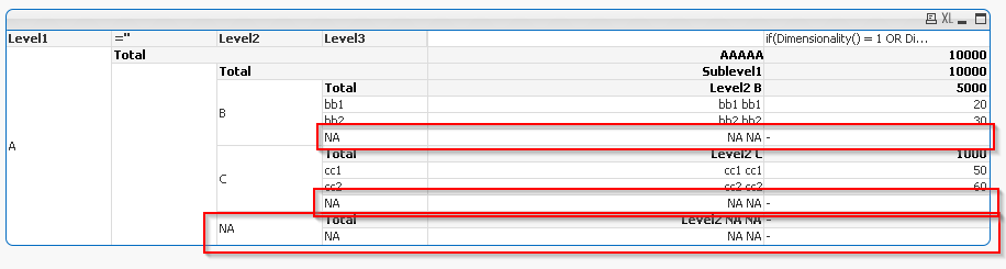
A have a data set like this:
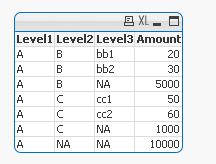
Notice the last row, where level2 is NA - this is actually a total for Level1.
Same is with NA in Level3 - these are the totals for given dimension value in Level2
Now I want to use this as a total in pivot table, but hide it from rows:
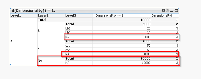
I want to hide what is marked in red.
Can someone help me with this please?
Thank you very much!
- « Previous Replies
-
- 1
- 2
- Next Replies »
Accepted Solutions
- Mark as New
- Bookmark
- Subscribe
- Mute
- Subscribe to RSS Feed
- Permalink
- Report Inappropriate Content
Here try this simple if statement
=If(Column(3) > 0,
if(Dimensionality()=1,Level1,
if(Dimensionality()=2,'A',
if(Dimensionality()=3,'B',
'C'
))))
- Mark as New
- Bookmark
- Subscribe
- Mute
- Subscribe to RSS Feed
- Permalink
- Report Inappropriate Content
PFA, I got like this?
- Mark as New
- Bookmark
- Subscribe
- Mute
- Subscribe to RSS Feed
- Permalink
- Report Inappropriate Content
This?
- Mark as New
- Bookmark
- Subscribe
- Mute
- Subscribe to RSS Feed
- Permalink
- Report Inappropriate Content
Hi, thanks. But totals disappear and are needed.
- Mark as New
- Bookmark
- Subscribe
- Mute
- Subscribe to RSS Feed
- Permalink
- Report Inappropriate Content
Hi Sunny,
this is great solution and I will probably mark it as Correct, but can you help me further please? Unfortunately i doesn't work for the structure of my pivot table which is required. And I cant figure out how to solve it. I have one more dimension between Levels, and one more expression. So I made an example which is a little closer. I kept the set analysis like it was done by you, just changed the dimensionality numbers.
And added dimension is just ='', which is used for the total displaying.
Please find the attached file.
What I would like, is to again get rid of the rows with NA:
Thank you very much 
- Mark as New
- Bookmark
- Subscribe
- Mute
- Subscribe to RSS Feed
- Permalink
- Report Inappropriate Content
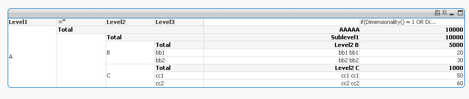
I think the problem was your 1st expression... try this
=if(Dimensionality()=1,
if(Level1='A','AAAAA'),
if(Dimensionality()=2,'Sublevel1',
if(Dimensionality()=3 and Level2 <> 'NA','Level2 '& Only({<Level2 -= {'NA'}>}Level2),
only({<Level2 -= {'NA'}, Level3 -= {'NA'}>}Level3)) & If(Level2 <> 'NA' and Level3 <> 'NA', ' ')&
only({<Level2 -= {'NA'}, Level3 -= {'NA'}>}Level3))
)
- Mark as New
- Bookmark
- Subscribe
- Mute
- Subscribe to RSS Feed
- Permalink
- Report Inappropriate Content
Beautiful
Thank you.
- Mark as New
- Bookmark
- Subscribe
- Mute
- Subscribe to RSS Feed
- Permalink
- Report Inappropriate Content
Hi Sunny,
I am a little ashamed right now, that I didn't give you all expressions I have, since there is one more which again made NA to appear. If you feel for another minor challenge or willing to help, here is what I have. And that's the last adage to the structure of pivot table
Please see the attachment.
There is an expression on second place, which has no label, and it just fills some strings based on dimensionality values.
Thank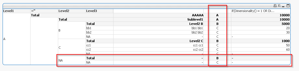
Thank you very much!
- Mark as New
- Bookmark
- Subscribe
- Mute
- Subscribe to RSS Feed
- Permalink
- Report Inappropriate Content
Here try this simple if statement
=If(Column(3) > 0,
if(Dimensionality()=1,Level1,
if(Dimensionality()=2,'A',
if(Dimensionality()=3,'B',
'C'
))))
- Mark as New
- Bookmark
- Subscribe
- Mute
- Subscribe to RSS Feed
- Permalink
- Report Inappropriate Content
OK, I think I made it work, by checking the Column 1 for NA. Seems good right now.
Thank you so much for help
- « Previous Replies
-
- 1
- 2
- Next Replies »