Unlock a world of possibilities! Login now and discover the exclusive benefits awaiting you.
- Qlik Community
- :
- All Forums
- :
- QlikView App Dev
- :
- Re: How to create a Bar Chart with multiple dimens...
- Subscribe to RSS Feed
- Mark Topic as New
- Mark Topic as Read
- Float this Topic for Current User
- Bookmark
- Subscribe
- Mute
- Printer Friendly Page
- Mark as New
- Bookmark
- Subscribe
- Mute
- Subscribe to RSS Feed
- Permalink
- Report Inappropriate Content
How to create a Bar Chart with multiple dimensions?
Hi,
My data looks something like this (a sample):
| CHEMICAL | SUPPLIER17 | 2.11 | 2.47 | 2.54 |
| CHEMICAL | SUPPLIER18 | 2.69 | 2.33 | 2.02 |
| CONSTRUCTION | SUPPLIER19 | 2.61 | 2.4 | 2.56 |
| CONSTRUCTION | SUPPLIER2 | 2.88 | 2.86 | 2.87 |
| CONSTRUCTION | SUPPLIER20 | 1.81 | 2.59 | 1.95 |
| CONSTRUCTION | SUPPLIER21 | 1.83 | 1.89 | 2.82 |
| CONSTRUCTION | SUPPLIER22 | 1.95 | 2.31 | 2.67 |
| CONSTRUCTION | SUPPLIER23 | 1.92 | 2.51 | 2.27 |
| CONSTRUCTION | SUPPLIER24 | 3.1 | 3.58 | 3.59 |
| METALWORKING | SUPPLIER25 | 3.45 | 3.29 | 3.06 |
| METALWORKING | SUPPLIER26 | 4.1 | 3.8 | 3.21 |
| METALWORKING | SUPPLIER27 | 4.24 | 3.2 | 3.6 |
I need a barchart that shows by each industry (Chemical/ Construction/ Metalworking) the names of suppliers (Supplier1, Supplier2 etc.) and their respective scores for each year (column 3,4,5 in the above table).. I'm only able to add Supplier Name & the respective score against each name, however, I'm not able to include the Industry name in the same chart, as, when I do so, the chart automatically changes to stacked type, which is not what I need.
I'm attaching my QV file.. could anyone please help with this?
Thanks,
Rajyalakshmi
- Tags:
- new_to_qlikview
- Mark as New
- Bookmark
- Subscribe
- Mute
- Subscribe to RSS Feed
- Permalink
- Report Inappropriate Content
Hi, I'm not sure if this is enough, but you can remove your dimension and include a calculated one with the following definition:
=INDUSTRY & '-' & [SUPPLIER NAME]
Hope it helps,
Erich
- Mark as New
- Bookmark
- Subscribe
- Mute
- Subscribe to RSS Feed
- Permalink
- Report Inappropriate Content
Hi Erich,
Thanks! This definitely helps.. But I was wondering if there was any way of getting the QV chart to look a little like the Excel version of the same chart :
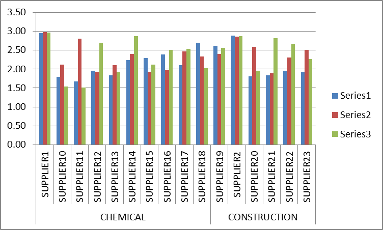
Please let me know if this is possible.. if not, would you suggest an alternate approach...?
Thanks,
RL