Pivot Table Conditional Formatting

[adamwigley]

Hi,

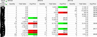
I have created a pivot table which looks at sales by product groups and compares data over the past 3 x years.  this was a report created in Excel they wanted me to recreate in Qlikview.  All OK accept that in Excel, they use conditional formatting to look at the latest average selling price and see if it is larger or smaller than the previous year.  This previous year's average selling price is then compared to the year before that, each time highlighting red if lower or green if above the previous years price.

I have no idea if Qlikview can do this or where I would start.

A screenshot of what my Qlikview application looks like is below, I have manually highlighted how I would want to use conditional formatting to highlight the data (in red and green):

Any help would be much appreciated.

Thanks,

Adam

[Kushal_Chawda · Accepted solution]

@adamwigley  try below background color expression for [Avg Price]

=if(after(total Your_Avg_Price_expression)<= Your_Avg_Price_expression, green(),red())

[adamwigley]

Hi @Kushal_Chawda,

Thanks for responding - the solution you provided worked perfectly! I just tweaked it to stop it from colouring everything in as per below:

=If(After(TOTAL [Avg Price]) > [Avg Price], LightRed()
,If(After(TOTAL [Avg Price]) < [Avg Price], LightGreen()))

Thanks again,

Adam