Rank Function Help

[alvinford]

Hi All ,

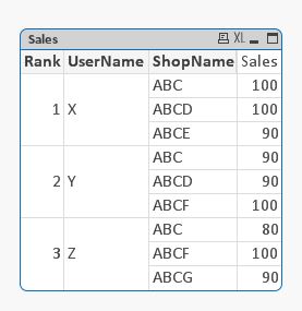
I have the below table , the requirement is to rank the UserName based on the sales value and display the first three UserNames as in the output shown below. Please help to get this requirement.

UserName	ShopName	SalesValue
X	ABC	100
Y	ABC	90
X	ABCD	100
Y	ABCD	90
X	ABCE	90
Y	ABCF	100
Z	ABC	80
Z	ABCG	90
V	AAA	80
Z	ABCF	100
V	ABC	80
U	ABB	70
V	ABCD	80
U	ABD	80
V	ABCF	20

Output

Rank	UserName	ShopName	SalesValue
1	X	ABC	100
		ABCD	100
		ABCE	90
2	Y	ABC	90
		ABCD	90
		ABCF	100
3	Z	ABC	80
		ABCG	90
		ABCF	100

Thanks & Regards,

Alvin

[MK_QSL]

Like this?

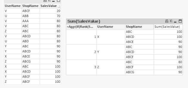
Create a pivot table

Dimension

1)

=Aggr(IF(Rank(SUM(Total<UserName>SalesValue))<=3,Rank(SUM(Total<UserName>SalesValue))),UserName)

Tick Suppress When Value is Null

2) UserName

3) ShopName

Expression

SUM(SalesValue)

[tresesco]

May be this?

Expression: =Aggr(If(Rank(Sum(SalesValue))<4, Rank(Sum(SalesValue))),UserName)

[alvinford]

Hi Tresesco,

Thank you for your reply. Its Working fine. Have other requirement on the top it. How can I display Top 2 ShopNames for the Top three ranks as I have more than one ShopNames

The Output expected is as below

Rank	UserName	ShopName	SalesValue
1	X	ABC	100
		ABCD	100
2	Y	ABCD	90
		ABCF	100
3	Z	ABCG	90
		ABCF	100

Thanks & Regards,

Alvin

[tresesco]

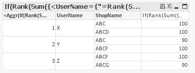
Use the expression like below:

If(Rank(Sum({<UserName={"=Rank(Sum(SalesValue))<4"}>}SalesValue),4)<3, Sum(SalesValue))

[alvinford]

Hi Tresesco,

Thank You Very much .. it worked for me ..