Rank in pivot table

[#1]

Hi everybody,

I have a pivot table with 2 dimensions, Quarter and Area and some expressions.

This pivot table is shown only when the user select only one company because there are some expressions about the market (= all companies) and some others about the selected company.

My pivot table is like this (dimensions in bold and expressions in italic)

Area                                                              Q1       Q2       Q3       Q4

North America      

  Sales Market                                              100     120     110     140

  Sales Selected Company                            30        40        25        50

  Rank Company                                            2          2          2          2                     

South America      

  Sales Market                                              110     125     130     140

  Sales Selected Company                            35        30        20        40

  Rank Company                                            1          1          1          1

Among my expressions, I need to calculate the rank but if I use this expression : =rank(sum({<$(CTXT_COMPANY),$(CTXT_REBATES)>}SALES)), the rank calculated is 1 or 2 because it’s calculated for only the selected company among Area.

I would like calculate the rank of the selected company among all companies, by area.

Could you help me for this ?

Thank you

Regards

Bérengère

[Gysbert_Wassenaar]

Try: rank(TOTAL sum({<$(CTXT_COMPANY),$(CTXT_REBATES)>}SALES))

[#3]

Hello Gysbert,

Thank you for your response. Unfortunately, I tried this and the result is the same.

Regards

Bérengère

[Gysbert_Wassenaar]

Can you post an example document that demonstrates the problem?

[#5]

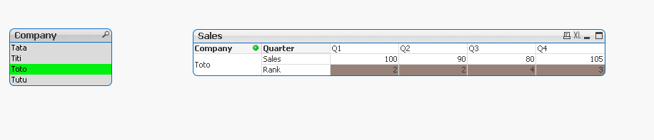
Here is an example of my problem.

Thank you

Regards

Bérengère

[Gysbert_Wassenaar]

Well, you can show the correct numbers with =rank(TOTAL sum({<Company>}Sales)). But then you will get all companies in the chart even if you select only one company in the list box.

[#7]

Yes but as you said, I get all companies in the pivot table and not only the selected company...

[Clever_Anjos]

Try this:

=if(Column(1) > 0,rank(TOTAL sum({<Company=>}Sales)))

[#9]

Hello Clever,

Thank you for your response. Results of expressions for others companies are 0 or null but they still appear in the pivot table.

Regards

Bérengère

[Clever_Anjos]

Weird... It worked here