Visual Effects Tab

[npadilla73]

Hello Community,

I have a pivot table with my production of the month, but I need identifying if my shift production reached their goal in the day.   So, in the Visual Effects Tab, in the option upper, I write down the field "Goal Production" , and do the same in the lower option.    But it does not work properly, because my expression remains in black color, but if I select only one ITEM,  the funtion works well.

Can someone tell me what I am doing wrong?

Thanks

I attached an example.

[stigchel]

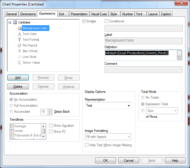
Instead of using the visual cues, use the background color option of the expression (click on the plus sign in front). There use

=if(Cantidad>[Goal Production],Green(),Red())

[npadilla73]

Thanks, that's exactly what I need.

[stigchel · Accepted solution]

You're welcome. You may want to add a rowno and/or secondarydimensionality condition to skip the totals from coloring, so

=IF(SecondaryDimensionality()>0,

if(Rowno()>0,if(Cantidad>[Goal Production],Green(),Red()))

)

Also if this has answered your question, could you mark the answer correct. It will close the thread helping others to find correct answers and let other contributing members know this requires no more attention

[npadilla73]

This sentence is better, thanks again.