Unlock a world of possibilities! Login now and discover the exclusive benefits awaiting you.
- Qlik Community
- :
- All Forums
- :
- QlikView App Dev
- :
- show top 2 rows of pivot based on expression deriv...
- Subscribe to RSS Feed
- Mark Topic as New
- Mark Topic as Read
- Float this Topic for Current User
- Bookmark
- Subscribe
- Mute
- Printer Friendly Page
- Mark as New
- Bookmark
- Subscribe
- Mute
- Subscribe to RSS Feed
- Permalink
- Report Inappropriate Content
show top 2 rows of pivot based on expression derived out of other expressions
Hello,
I have a pivot table as mentioned below with 3 expressions.
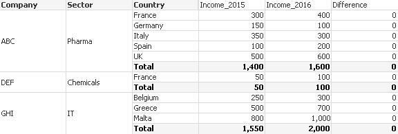
Difference is the difference in income between 2016 & 2015. I want to show only 2 companies with highest increase in revenue in 2016 compared to 2015.
I tried using the expression: =Sum({<Company={"=Rank(([Income_2016]-[Income_2015]),4)<=2"}>}Income) but it's not working.
Can you please help.
With regards,
Ayandeep
Accepted Solutions
- Mark as New
- Bookmark
- Subscribe
- Mute
- Subscribe to RSS Feed
- Permalink
- Report Inappropriate Content
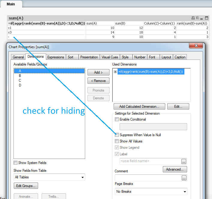
Hi, Ayandeep!
This could be achieved with calculated dimension in pivot table.
For instance, you have a table:
LOAD * Inline
[A,B,C,D
10,12,13,x1
9,10,11,x2
14,18,18,x3];
Where "D" is a companies and a "Column(2)-Column(1)" is a difference you need. Next you may follow this picture:
- Mark as New
- Bookmark
- Subscribe
- Mute
- Subscribe to RSS Feed
- Permalink
- Report Inappropriate Content
Is Income_2016 expression label or the expression/field itself? If it is expression label, then I doubt it will work within set analysis. Use the actual expressions here:
=Sum({<Company={"=Rank((2016 Income Expression - 2015 Income Expression),4)<=2"}>}Income)
- Mark as New
- Bookmark
- Subscribe
- Mute
- Subscribe to RSS Feed
- Permalink
- Report Inappropriate Content
Hi Sunny,
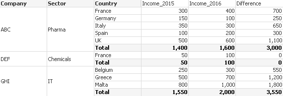
It's the expression label. So i tried using the actual expression as mentioned below.
=Sum({<Company={"=Rank((Sum({<Year={2016}>}Income)-Sum({<Year={2015}>}Income)),4)<=2"}>}Income)
But instead of subtracting it is creating a summation.
- Mark as New
- Bookmark
- Subscribe
- Mute
- Subscribe to RSS Feed
- Permalink
- Report Inappropriate Content
Try this
=Sum({<Company={"=Rank((Sum({<Year={2016}>}Income)-Sum({<Year={2015}>}Income)),4)<=2"}, Year={2016}>}Income)
-Sum({<Company={"=Rank((Sum({<Year={2016}>}Income)-Sum({<Year={2015}>}Income)),4)<=2"}, Year={2015}>}Income)
- Mark as New
- Bookmark
- Subscribe
- Mute
- Subscribe to RSS Feed
- Permalink
- Report Inappropriate Content
Hi, Ayandeep!
This could be achieved with calculated dimension in pivot table.
For instance, you have a table:
LOAD * Inline
[A,B,C,D
10,12,13,x1
9,10,11,x2
14,18,18,x3];
Where "D" is a companies and a "Column(2)-Column(1)" is a difference you need. Next you may follow this picture:

- Mark as New
- Bookmark
- Subscribe
- Mute
- Subscribe to RSS Feed
- Permalink
- Report Inappropriate Content
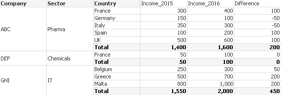
With this expression I am getting the difference but it's showing all 3 Companies only with the value of the 3rd as 0. Please refer below image.
- Mark as New
- Bookmark
- Subscribe
- Mute
- Subscribe to RSS Feed
- Permalink
- Report Inappropriate Content
Thanks Sergey. Works exactly as per requirement ![]()
- Mark as New
- Bookmark
- Subscribe
- Mute
- Subscribe to RSS Feed
- Permalink
- Report Inappropriate Content
Hi,
Script:
Year(Date) as Year1,
Dimension:
=if(aggr(rank(aggr(sum({<Year1={2016}>}Income),Company,Sector)-
aggr(sum({<Year1={2015}>}Income),Company,Sector)),Company)<=2,Company)
=Sector
=Country
Expression:
=sum({<Year1={2016}>}Income)
=sum({<Year1={2015}>}Income)
Regards,
Sanya Chauhan
- Mark as New
- Bookmark
- Subscribe
- Mute
- Subscribe to RSS Feed
- Permalink
- Report Inappropriate Content
Although you got the answer you wanted, but just to explain what you went wrong here... You wanted to remove the rows where rank was greater than 2, right? But only your third expression was showing 0, rest of the two expressions were still showing a non-zero numbers. So what can you do to make those rows 0 also? Use an if statement like this
(assuming Difference is your third expression)
Expression1:
Sum({<Company={"=Rank((Sum({<Year={2016}>}Income)-Sum({<Year={2015}>}Income)),4)<=2"}, Year={2015}>}Income)
Expression2:
If(Column(3) > 0, Sum({<Company={"=Rank((Sum({<Year={2016}>}Income)-Sum({<Year={2015}>}Income)),4)<=2"}, Year={2016}>}Income))
Expression3:
=Sum({<Company={"=Rank((Sum({<Year={2016}>}Income)-Sum({<Year={2015}>}Income)),4)<=2"}, Year={2016}>}Income)
-Sum({<Company={"=Rank((Sum({<Year={2016}>}Income)-Sum({<Year={2015}>}Income)),4)<=2"}, Year={2015}>}Income)
Now what the expression1 and expression2 if statement will do is that it will make above rank 2 rows as 0 also and those rows will automatically suppress (if you have checked 'Suppress Zero Value' on the presentation tab)
Just as a side note, set analysis is a better performant then calculated dimension (almost every time).
Best,
Sunny