Unlock a world of possibilities! Login now and discover the exclusive benefits awaiting you.
- Qlik Community
- :
- All Forums
- :
- QlikView App Dev
- :
- Calculated dimension in pivot table to show status...
- Subscribe to RSS Feed
- Mark Topic as New
- Mark Topic as Read
- Float this Topic for Current User
- Bookmark
- Subscribe
- Mute
- Printer Friendly Page
- Mark as New
- Bookmark
- Subscribe
- Mute
- Subscribe to RSS Feed
- Permalink
- Report Inappropriate Content
Calculated dimension in pivot table to show status history
Hi there,
I have some data for project reportings and would like to show a pivot table like this one:
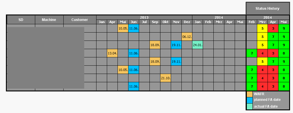
So far this table are in fact two tables. The status history on the right hand side is a second pivot table. That's not want I want especially when it comes to scrolling the table.
Besides the other data I have the status history in an excel file as shown below. 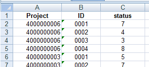
Every month we have to report our projects, so every ID equals one month.
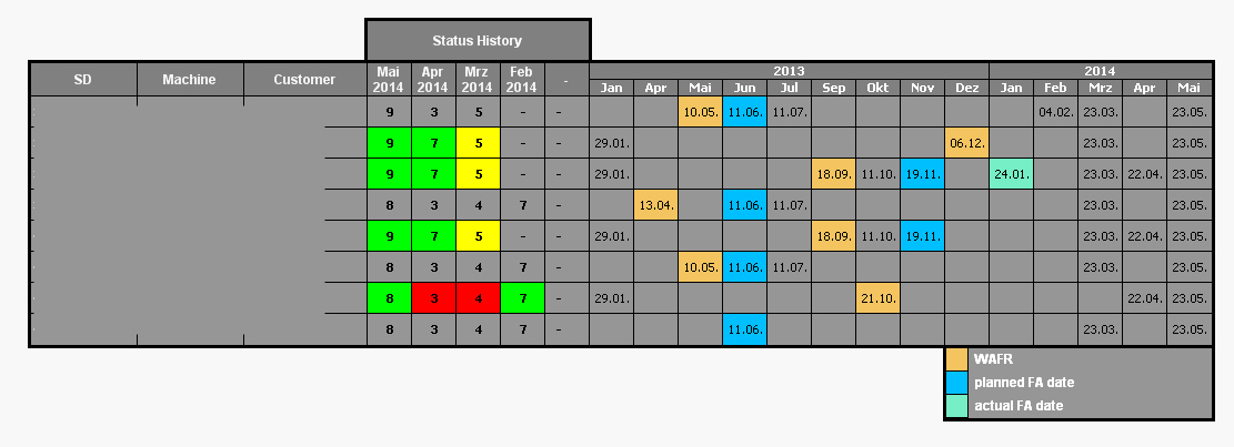
What I want to do is to join both tables, while the Status history should always show the last six entries.
However, I guess I would need a calculated dimension for each of the last six entries to exactly pick one status per column.
I don't know whats wrong, but I only works for one column or entry. Everytime I create a calculated domension for the second entry it stays empty. In my first column I can show all of the last six entries by simply changing the dimension (for example using rank() in the dimension to swap form entry to entry) but I need to show all six in seperate columns as shown in the first screenshot.
Can anybody help?
Thanks and best regards,
Christian
Accepted Solutions
- Mark as New
- Bookmark
- Subscribe
- Mute
- Subscribe to RSS Feed
- Permalink
- Report Inappropriate Content
Perhaps you can use the firstsortedvalue function to get the status you want. Something like =aggr(firstsortedvalue(status, -ID), SD, Machine, Customer)
=aggr(firstsortedvalue(status, -ID, 2), SD, Machine, Customer)
...
=aggr(firstsortedvalue(status, -ID, 6), SD, Machine, Customer)
talk is cheap, supply exceeds demand
- Mark as New
- Bookmark
- Subscribe
- Mute
- Subscribe to RSS Feed
- Permalink
- Report Inappropriate Content
Hey Gysbert,
yeah - it works 
I already tried firstsortedvalue, but didn't use the aggr() function. That did the trick.
There is just one thing I don't get: I would like to color the background of the cells according to their values.
This is my (shortened) function:
=if(aggr(firstsortedvalue(Gesamtstatus, -ID),SD,Maschine, Kunde)>6, rgb(0,255,0), rgb(150,150,150))
Strange thing is that it only works if there is an entry in the first date field right beside the status history:
It does not work for the other entries until I select only one of them:
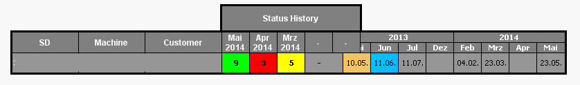
I don't know why but the fields seem to be related somehow.
Do you have an idea how I could solve that?
Thanks a lot and best regards,
Christian