Unlock a world of possibilities! Login now and discover the exclusive benefits awaiting you.
- Qlik Community
- :
- All Forums
- :
- QlikView App Dev
- :
- Problem with Formatting text color in pivot table ...
- Subscribe to RSS Feed
- Mark Topic as New
- Mark Topic as Read
- Float this Topic for Current User
- Bookmark
- Subscribe
- Mute
- Printer Friendly Page
- Mark as New
- Bookmark
- Subscribe
- Mute
- Subscribe to RSS Feed
- Permalink
- Report Inappropriate Content
Problem with Formatting text color in pivot table with conditional expression
Hi everyone,
I have a pivot table, like below
| April | May | June | |
|---|---|---|---|
| class1 | 100 | 200 | 100 |
| class2 | 50 | 25 | 30 |
| class 3 | 45 | 15 | 12 |
the number in the middle will be called Amount and its sum
Lets say i want to be able to test one and only 1 cell of this table regarding its values, compare it to a lower and higher value and change the color depending on when this value is situated
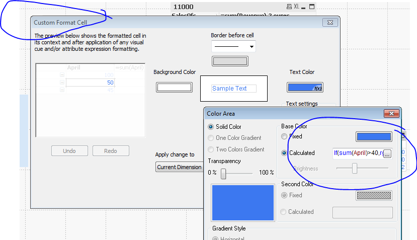
For instance, i want to check the April Class 2. If the value is bigger than 55 then it goes RED, if it is lower than 40, it goes GREEN, else it goes amber. Right now the Value is 50 so it should be YELLOW.
on the calculated expression of that pivot, i click on the + , went to Text Color , and applied the following expression :
if ( Month = 'April' ,
if ( class = 'class2'
if ( Amount > 55, red(),
if ( Amount < 40 , green(),
yellow()
)
)
)
)
The result is : that number is always Green .... no matter what i do, so it means that it jumped to the second if .
I tried a lot of possibilities with my formula, and i never be able to make it.
Anyone to help ?
thanks a lot
- Mark as New
- Bookmark
- Subscribe
- Mute
- Subscribe to RSS Feed
- Permalink
- Report Inappropriate Content
Can you post a qlikview document that demonstrates the problem?
talk is cheap, supply exceeds demand
- Mark as New
- Bookmark
- Subscribe
- Mute
- Subscribe to RSS Feed
- Permalink
- Report Inappropriate Content
can u try some thing like this,