Unlock a world of possibilities! Login now and discover the exclusive benefits awaiting you.

- Qlik Community
- :
- All Forums
- :
- QlikView
- :
- Re: Pivot Chart Help - Conditions
- Subscribe to RSS Feed
- Mark Topic as New
- Mark Topic as Read
- Float this Topic for Current User
- Bookmark
- Subscribe
- Mute
- Printer Friendly Page

- Mark as New
- Bookmark
- Subscribe
- Mute
- Subscribe to RSS Feed
- Permalink
- Report Inappropriate Content
Pivot Chart Help - Conditions
Hello,
Looking for help on the Pivot Table dimension shown below
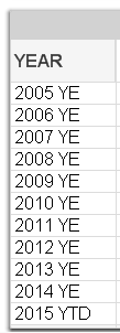
I am using the following calculated dimension:
=IF(YEAR < $(vBusinessYear) , YEAR & ' YE', YEAR & ' YTD' )
I would like to get rid of 2005-2007 on the graph as I only need >= 2008. I am also looking to have this table static to always show each year, so I have YEAR =, in the set analysis. Is there a way to change the calculated dimension or use the conditional setting? I have tried several options with no luck.
Thank you,
Justin
Accepted Solutions

 sunny_talwar
- Mark as New
- Bookmark
- Subscribe
- Mute
- Subscribe to RSS Feed
- Permalink
- Report Inappropriate Content
Did you try this by any chance?
=If(YEAR >= 2008, IF(YEAR < $(vBusinessYear) , YEAR & ' YE', YEAR & ' YTD'))
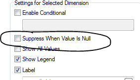
Update: and ensure that you have suppressed the null value for the calculated dimension.
Best,
Sunny
sunny_talwar
- Mark as New
- Bookmark
- Subscribe
- Mute
- Subscribe to RSS Feed
- Permalink
- Report Inappropriate Content
Did you try this by any chance?
=If(YEAR >= 2008, IF(YEAR < $(vBusinessYear) , YEAR & ' YE', YEAR & ' YTD'))
Update: and ensure that you have suppressed the null value for the calculated dimension.
Best,
Sunny
- Mark as New
- Bookmark
- Subscribe
- Mute
- Subscribe to RSS Feed
- Permalink
- Report Inappropriate Content
I thought I had, but apparently I did not.
Thanks for the help,
Justin
sunny_talwar
- Mark as New
- Bookmark
- Subscribe
- Mute
- Subscribe to RSS Feed
- Permalink
- Report Inappropriate Content
So did it work now?
Best,
Sunny
- Mark as New
- Bookmark
- Subscribe
- Mute
- Subscribe to RSS Feed
- Permalink
- Report Inappropriate Content
Sure does Sunny, thank you again.
sunny_talwar
- Mark as New
- Bookmark
- Subscribe
- Mute
- Subscribe to RSS Feed
- Permalink
- Report Inappropriate Content
Awesome!, glad to help.
Best,
Sunny