Unlock a world of possibilities! Login now and discover the exclusive benefits awaiting you.
- Qlik Community
- :
- Forums
- :
- Analytics & AI
- :
- Products & Topics
- :
- Visualization and Usability
- :
- How to add a row calculating difference on a pivot...
- Subscribe to RSS Feed
- Mark Topic as New
- Mark Topic as Read
- Float this Topic for Current User
- Bookmark
- Subscribe
- Mute
- Printer Friendly Page
- Mark as New
- Bookmark
- Subscribe
- Mute
- Subscribe to RSS Feed
- Permalink
- Report Inappropriate Content
How to add a row calculating difference on a pivot table?
Hello,
In QlikSense, how can I add an additional row to my Pivot Table calculating the difference between the rows above it? I've searched all around and can't find how to do it as a row below my other rows.
I'm not looking to add the difference as a column to the right.
I want it to look just like the red text in this image:
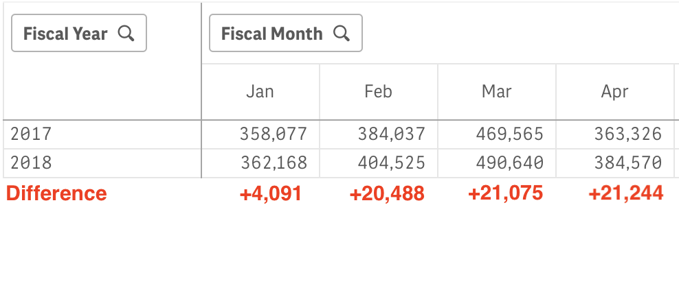
Thanks!
Accepted Solutions
- Mark as New
- Bookmark
- Subscribe
- Mute
- Subscribe to RSS Feed
- Permalink
- Report Inappropriate Content
can't do that. you need to create separate Measures (Measure 1: 2017, 2: 2018, 3: 2017-2017) (so not using year as a dimension)
- Mark as New
- Bookmark
- Subscribe
- Mute
- Subscribe to RSS Feed
- Permalink
- Report Inappropriate Content
can't do that. you need to create separate Measures (Measure 1: 2017, 2: 2018, 3: 2017-2017) (so not using year as a dimension)
- Mark as New
- Bookmark
- Subscribe
- Mute
- Subscribe to RSS Feed
- Permalink
- Report Inappropriate Content
Thank you for the straightforward answer. The inability of Qliksense to do simple operations can be extremely frustrating.
- Mark as New
- Bookmark
- Subscribe
- Mute
- Subscribe to RSS Feed
- Permalink
- Report Inappropriate Content
... Qlik Sense is not Excel...
dimensions cannot be added/multiplied/... only measures can...
- Mark as New
- Bookmark
- Subscribe
- Mute
- Subscribe to RSS Feed
- Permalink
- Report Inappropriate Content
did you find a way to achieve what you wanted nathan?
- Mark as New
- Bookmark
- Subscribe
- Mute
- Subscribe to RSS Feed
- Permalink
- Report Inappropriate Content
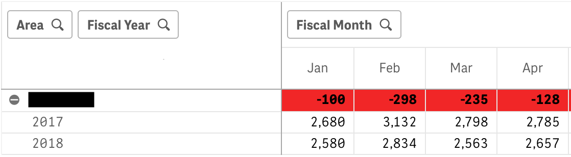
I got close to the desired result by using the method described here: Calculate Difference in Rows in Pivot
Unfortunately, it requires the user click a "disclosure" widget to open the upper level before the lower level can display. That makes it likely my customer will not see the detail I want them to see, since they are unlikely to interact with the worksheet.
It also places the total above the rows, which is counter-intuitive, but functional.
the sheet opens looking like this:

and expands to this:
I accept that Qlik Sense is not Excel, but its inflexible reporting and limited data graphics capabilities make it difficult. But since my company has decided it will be our one and only reporting platform, it is what I must work with.
- Mark as New
- Bookmark
- Subscribe
- Mute
- Subscribe to RSS Feed
- Permalink
- Report Inappropriate Content
@nlee4jnj please, can i have sample of how you did it?
- Mark as New
- Bookmark
- Subscribe
- Mute
- Subscribe to RSS Feed
- Permalink
- Report Inappropriate Content
I recommend you read the post I linked to. Basically, I used the DIMENSIONALITY() function, which lets you calculate differently based on whether the pivot table row is a header row or a dimension detail row.
Basically, it's this:
IF(Dimensionality()=1, **SUM GOES HERE**)
    ,
    DIMENSION MEASURE GOES HERE)
)
Then I used the Styling options for the Pivot Table to make it expanded at all times.

- Mark as New
- Bookmark
- Subscribe
- Mute
- Subscribe to RSS Feed
- Permalink
- Report Inappropriate Content
This challenge is already a show stopper for us at Para Systems Ltd. Customer has insisted on getting value for their investment in Qliksense otherwise maintenance support contract proposition will not fly.
Marcel's concern on multiple row calculation.
It is an issue that Qlik should support us to resolve to earn continued patronage of the customer.
There are several opportunities in the Oil & Gas sector to be exploited.
Your support is very crucial please