Unlock a world of possibilities! Login now and discover the exclusive benefits awaiting you.
- Qlik Community
- :
- All Forums
- :
- QlikView App Dev
- :
- pivot table use different dimension for total
- Subscribe to RSS Feed
- Mark Topic as New
- Mark Topic as Read
- Float this Topic for Current User
- Bookmark
- Subscribe
- Mute
- Printer Friendly Page
- Mark as New
- Bookmark
- Subscribe
- Mute
- Subscribe to RSS Feed
- Permalink
- Report Inappropriate Content
pivot table use different dimension for total
Hello,
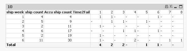
I'm trying to implement a pivot table which has the same appearance as this table:
Two dimensions: ship week and Time2Fail
| Time2Fail | 1 | 2 | 3 | 4 | 5 | 6 | 7 | 8 | ||
| ship week | ship count | Accu ship count | ||||||||
| 1 | 4 | 4 | 1 | 1 | 1 | |||||
| 2 | 5 | 9 | 1 | 1 | 1 | |||||
| 3 | 2 | 11 | 1 | |||||||
| 4 | 6 | 17 | 1 | 1 | 1 | |||||
| 5 | 2 | 19 | 1 | |||||||
| 6 | 11 | 30 | 1 | 2 | 1 | 1 | ||||
| 3 | 3 | 2 | 0 | 1 | 1 |
expression1: The ship count is how many units shipped in a ship week.
expression2: The Accu Ship count is the accumulate ship count along the the ship week.
e.g. accu ship count for ship week 1 is 4, for ship week 2 is 4+5=9 and for ship week 3 is 9+2= 11 and so on
expression3: The last row is the sub total of the column Time2Fail, but only count up to the ship week.
e.g. for the Time2Fail = 1 column, sub total = 1+1+1 = 3 (to ship week = 6)
for the Time2Fail = 2 column, sub total = 1+1+1 = 3 (to ship week = 5)
for the Time2Fail = 3 column, sub total = 1 +1=2 (to ship week = 4)
for the Time2Fail = 4 column, sub total = 0 (to ship week = 3)
for the Time2Fail = 5 column, sub total = 1 (to ship week = 2)
for the Time2Fail = 6 column, sub total = 1 (to ship week = 1)
based on the data:
| ship week | ID | Time2Fail |
| 1 | 1000 | 1 |
| 1 | 1001 | 2 |
| 1 | 1002 | |
| 1 | 1003 | 6 |
| 2 | 1954 | 3 |
| 2 | 1958 | |
| 2 | 1959 | 2 |
| 2 | 1967 | |
| 2 | 1988 | 5 |
| 3 | 2845 | 1 |
| 3 | 2846 | |
| 4 | 1323 | 3 |
| 4 | 1325 | |
| 4 | 1427 | 4 |
| 4 | 1377 | |
| 4 | 1388 | |
| 4 | 1399 | 6 |
| 5 | 6778 | 1 |
| 5 | 6779 | |
| 6 | 6770 | 1 |
| 6 | 8912 | |
| 6 | 1345 | 4 |
| 6 | 4523 | |
| 6 | 4524 | |
| 6 | 9923 | |
| 6 | 9924 | 7 |
| 6 | 9925 | |
| 6 | 9926 | 4 |
| 6 | 9927 | |
| 6 | 9928 | 8 |
Thanks,
Josh
- Tags:
- qlikview_scripting
- « Previous Replies
-
- 1
- 2
- Next Replies »
Accepted Solutions
- Mark as New
- Bookmark
- Subscribe
- Mute
- Subscribe to RSS Feed
- Permalink
- Report Inappropriate Content
This?
Expression:
=If(Dimensionality() = 0,
Sum(Aggr(If(Max(TOTAL [ship week]) - Time2Fail + 1 >= [ship week], Count(ID)), [ship week], Time2Fail)),
Count(ID))
- Mark as New
- Bookmark
- Subscribe
- Mute
- Subscribe to RSS Feed
- Permalink
- Report Inappropriate Content
Not sure I understand expression 3, but is this what you wanted?

- Mark as New
- Bookmark
- Subscribe
- Mute
- Subscribe to RSS Feed
- Permalink
- Report Inappropriate Content
Sunny T,
It's a wonderful answer except for expression 3. Thank you so much.
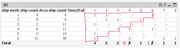
The expression 3 means the total is the partial total for those fall inside a step shape as depicted in the red line. So the total for column Time2Fail 4 should be 0 and 1 for column Time2Fail 6.
It will be appreciated if you can also provide an answer for expression 3.
Best,
Josh
- Mark as New
- Bookmark
- Subscribe
- Mute
- Subscribe to RSS Feed
- Permalink
- Report Inappropriate Content
I see what you mean. Let me play around with it 
- Mark as New
- Bookmark
- Subscribe
- Mute
- Subscribe to RSS Feed
- Permalink
- Report Inappropriate Content
This?
Expression:
=If(Dimensionality() = 0,
Sum(Aggr(If(Max(TOTAL [ship week]) - Time2Fail + 1 >= [ship week], Count(ID)), [ship week], Time2Fail)),
Count(ID))
- Mark as New
- Bookmark
- Subscribe
- Mute
- Subscribe to RSS Feed
- Permalink
- Report Inappropriate Content
Sunny T,
You are amazing!
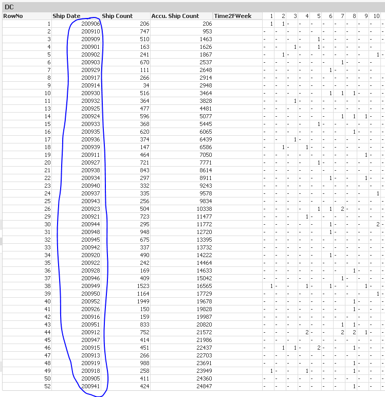
Now I'm implementing the answer your provide to our actual data.
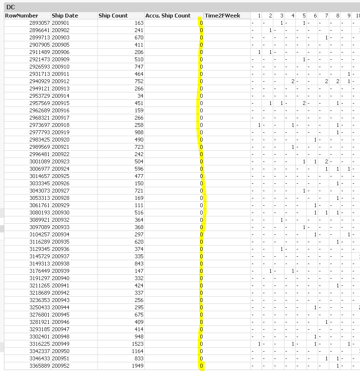
Turn out, the Accu Ship Count doesn't follow the the order of Ship Date.
More precise, the RowNo numbering is not based on the sorting order of Ship Date.
Here is a screenshot:
How to fix it?
Appreciate in advance.
Josh
- Mark as New
- Bookmark
- Subscribe
- Mute
- Subscribe to RSS Feed
- Permalink
- Report Inappropriate Content
I would suggest to fix this in the script.
FactTable:
LOAD [Ship Date],
....
FROM Source;
LinkTable:
LOAD Distinct [Ship Date],
RowNo() as RowNo
Resident FactTable
Order By [Ship Date];
So, essentially create RowNo() in a new table where you order your Ship Date in ascending order.
HTH
Best,
Sunny
- Mark as New
- Bookmark
- Subscribe
- Mute
- Subscribe to RSS Feed
- Permalink
- Report Inappropriate Content
Sunny T,
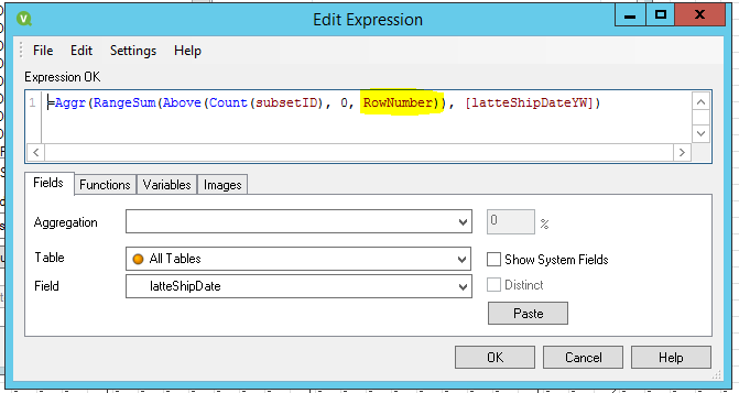
It's not working well if I use RowNo generated in script.
I used "RowNo() AS RowNumber" instead of "RowNo() AS RowNo" as described in your solution.
And I made the change accu. Ship Count expression according to the change from RowNo to RowNumber.
In our case, the table I showed you earlier actually is a result of filtering by couple list boxes.
The original table has thousands record. So, after filtering, the RowNumber is not contiguous and not starting from 1.
Here is the result. All 0's for Accu. Ship Count
- Mark as New
- Bookmark
- Subscribe
- Mute
- Subscribe to RSS Feed
- Permalink
- Report Inappropriate Content
Would you be able to share the new application to take a look at?
- Mark as New
- Bookmark
- Subscribe
- Mute
- Subscribe to RSS Feed
- Permalink
- Report Inappropriate Content
I can share the qvw but don't know how to attach.
- « Previous Replies
-
- 1
- 2
- Next Replies »