Unlock a world of possibilities! Login now and discover the exclusive benefits awaiting you.
- Qlik Community
- :
- Blogs
- :
- Technical
- :
- Design
- :
- Monte Carlo Methods
- Subscribe to RSS Feed
- Mark as New
- Mark as Read
- Bookmark
- Subscribe
- Printer Friendly Page
- Report Inappropriate Content
In some situations in Business Intelligence you need to make simulations, sometimes referred to as "Monte Carlo methods". These are algorithms that use repeated random number sampling to obtain approximate numerical results. In other words – using a random number as input many times, the methods calculate probabilities just like actually playing and logging your results in a real casino situation: hence the name.
These methods are used mainly to model phenomena with significant uncertainty in inputs, e.g. the calculation of risks, the prices of stock options, etc.
QlikView is very well suited for Monte Carlo simulations.
The basic idea is to generate data in the QlikView script using the random number generator Rand() in combination with a Load … Autogenerate, which generates a number of records without using an explicit input table.
To describe your simulation model properly, you need to do some programming in the QlikView script. Sometimes a lot. However, this is straightforward if you are used to writing formulae and programming code, e.g. Visual Basic scripts.
The Rand() function creates a uniformly distributed random number in the interval [0,1], which probably isn’t good enough for your needs: You most likely need to generate numbers that are distributed according to some specific probability density function. Luckily, it is in many cases not difficult to convert the result of Rand() to a random number with a different distribution.
The method used for this is called Inverse Transform Sampling: Basically, you take the cumulative probability function of the distribution, invert it, and use the Rand() function as input. See figure below.
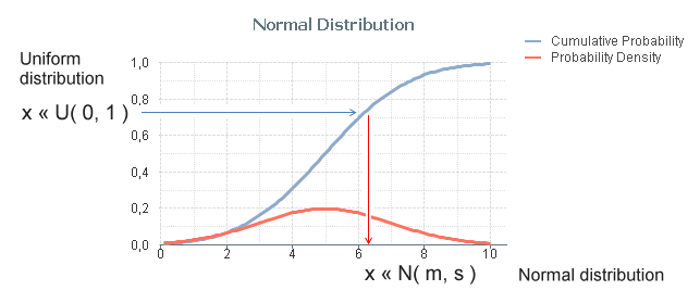
The most common probability distributions already exist in QlikView as inverse cumulative functions; Normal T, F and Chi-squared. Additional functions can be created with some math knowledge. The following definitions can be used for the most common distributions:
- Normal distribution: NormInv( Rand(), m, s )
- Log-Normal distribution: Exp( NormInv( Rand(), m, s ))
- Student's T-distribution: TInv( Rand(), d )
- F-distribution: FInv( Rand(), d1, d2 )
- Chi-squared distribution: ChiInv( Rand(), d )
- Exponential distribution: -m * Log( Rand() )
- Cauchy distribution: Tan( Pi() * (Rand()-0.5) )
Finally, an example that shows the principles around Monte Carlo methods: You want to estimate π (pi) using a Monte Carlo method. Then you could generate an arbitrary position x,y where both x and y are between 0 and 1, and calculate the distance to the origin. The script would e.g. be:
Load *,
Sqrt(x*x + y*y) as r;
Load
Rand() as x,
Rand() as y,
RecNo() as ID
Autogenerate 1000;
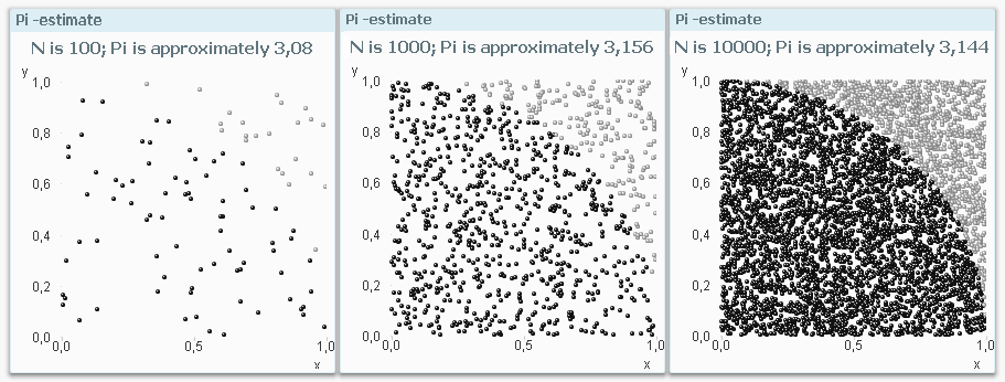
The ratio between the number of instances that are within one unit of distance from the origin and the total number of instances should be π/4. Hence π can be estimated through 4*Count( If(r<=1, ID)) / Count(ID).
Bottom line: Should you need to make Monte Carlo simulations – don’t hesitate to use QlikView. You will be able to do quite a lot.
See also the Tech Brief on how to generate data.
- « Previous
-
- 1
- 2
- 3
- Next »
You must be a registered user to add a comment. If you've already registered, sign in. Otherwise, register and sign in.