Challenge: Adjust table according to week filter

[gorterzelf7]

I got a real challenge for you guys. I really hope somebody is going to help me, please be my guest and try to build it yourself.

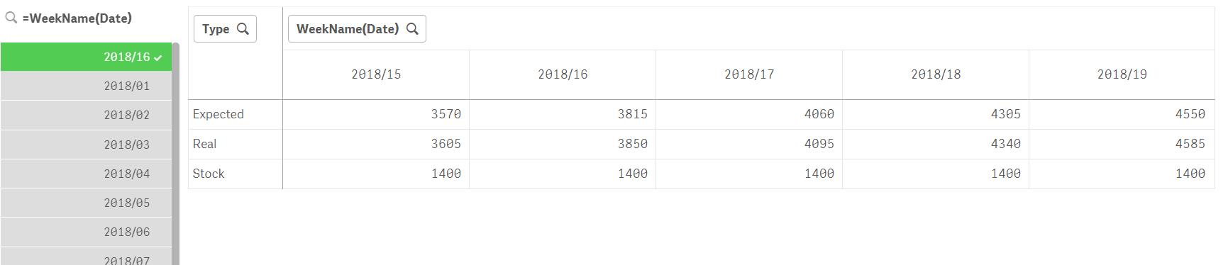
I have added the source and the wanted outcome, which should speak for itself but some extra text below.

I want to have a filter with the week. If you select a week, you should see that week in the outcome including -1 week and + 3 weeks. (like the example). If you selected a week below current week it should take next year. It is not needed to select father then one year from now. There is also a challenge when you select for example week 51, then i would like to see week 50, 51, 52, 1 and 2.

I think it shoud be like 5 expressions, with a formula but have not figured out how, but any other idea is welcome.

I really hope anybody is able to show me how this could be done in QlikSense, you can sent me the app or an example of the formulas.

If you have any questions, please do not hesitate to ask.

Kind Regards Martijn

[petter · Accepted solution]

Here is something that is quite close to what you are looking for I believe. You just have to tweak the expressions and possibly the weekstart day to finetune it. I leave that to you:

[gorterzelf7]

Thank you so very much Petter. I was lookging all day yesterday if somebody answered but your answer, just popped up this morning.

I have 2 additional questions:

1) Can i do this without the crosstable in the script, because my original script is very long with a very long linktable.

So would be nice if i do not have to change that.

2) Can the results also be presented in a straight table, because i wanna use lots of conitional formating, that is not available in the pivot table at the moment.

I really appreciate your help, you have no idea how much;-)

[petter]

1. It is even easier load script wise... just keep the source table format(s). Note: A CrossTable operation is very efficient and the table format you get is more tuned for analysis and BI puposes. I think keeping the format is less efficient but I do understand that with link-tables it could be a bit more complicated to handle.
2. Yes that is also relatively easy.

    a) You will have to have a synthetic dimension to give the rows for the Expected, Real and Stock:

                =ValueList('Expected','Real','Stock')

    b) You will have to create five measures with a Pick() and Match() combination to get the right sum

          according to which row that is displayed. For the first measure it will look like this:

Pick( Match( ValueList('Expected','Real','Stock'), 'Expected','Real','Stock')

  ,Sum( {1<Date={">=$(=WeekStart(Min(Date),-1,0))<=$(=WeekEnd(Min(Date),-1,0))"}>} Expected)

  ,Sum( {1<Date={">=$(=WeekStart(Min(Date),-1,0))<=$(=WeekEnd(Min(Date),-1,0))"}>} Real)

  ,Sum( {1<Date={">=$(=WeekStart(Min(Date),-1,0))<=$(=WeekEnd(Min(Date),-1,0))"}>} Stock)

)

For the next four measures you only have to change the bolded -1 in the above expression to the 0,1,2 and 3.

I have attached an updated version of the app.

[gorterzelf7]

I would like to thank you very much, I thought I knew quite a bit, but it turns out that I do not know that much at all.

I tried your formula, which works perfectly, but have not completely figured it out yet, in my situation.

I am a little embarred, but i think i have not explained it well, wondered if you could take a look at it. It is totally my fault, but i think we are very close, i changed the source and the outcome in the enclosed documents. Could you please consider taking another look at it. I am really, really, happy with your help petter-s

Sincerely, Martijn

[gorterzelf7]

Hello Petter, I am a little embarrased that i did not explain it well, but did you see my latest answer? I am really curious if there is way to fix it. Tnx again. Martijn

[petter]

Yes - it is possible to do it. The Pivot Table would probably be quicker to use development-wise. It would be to extend what I already have shown you.

[petter]

By the way - your Excel sheet for SourceNew.xlsx has an error in it... line 643 in fact. And the source data is not very well suited for testing as all numbers are the same for different years so it is hard to determine when developing whether you have the expressions right....

[gorterzelf7]

Ok, thank you for your fast answer Petter, I changed the source and it should be better now.

This seems to work for the current week. Any idea how I can take 1 year off?

IF(Origin='Expected',

NUM(Sum( {1<Date={">=$(=WeekStart(Min(Date),-1,0))<=$(=WeekEnd(Min(Date),-1,0))"}>} Amount)/

Sum( {1<Date={">=$(=WeekStart(Min(Date),-1,0))<=$(=WeekEnd(Min(Date),-1,0))"}>} Amount1), '€ #.##0,000;€ #.##0,000-' )

I have also thought about the pivot table:

1) I think I should make a new table with my linktable as the source?

2) Can I add 2 amounts and lot of dimensions? in the pivot table script?

3) I don't want to use a pivot table in the outcome, there i want a straight table because of the conditional formating. Is that possible?

I hope you understand what i mean?

Greetings Martijn

[petter]

There is an AddYears() function tou can use.