App Development

[aknabe1]

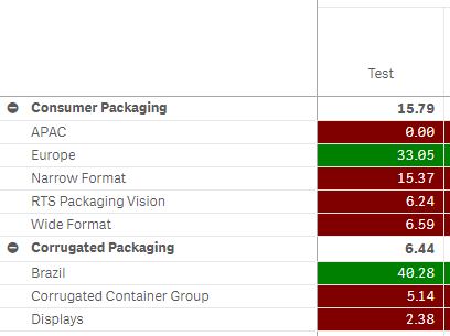
Is it possible to compare the second level of a pivot table (dimensionality = 2) to its parent value (dimensionality = 1).  In the image below, I am looking to compare the values that fall under "consumer packaging" to values that fall underneath. For example, compare APAC (0.00) to Consumer Packaging (15.79), Europe (33.05) to Consumer Packaging (15.79), etc... 

I have tried using the formula below but need to compare to a dynamic value opposed to a constant ( >20). 

=if(Dimensionality() = 2, if(( Test) > 20 ,green(), red()))

[edwin]

if what you want is to compare the result for the parent against the child, you can use aggregate.  and assuming you dont want the parent highlighted:

if(Dimensionality()>1, if( yourExpressionHere > AGGR(yourExpressionHere, parentFieldHere), green(), red()))

for example if your fields are CATEGORY as dimension1 and MEASURE as your value:

if(Dimensionality()>1, if(avg(MEASURE) > AGGR( avg(MEASURE), [CATEGORY]), green(), red()))

hope that makes sense

[edwin]

of course you need to decide if its a >= comparison - whats the color when the same

[vinieme12 · Accepted solution]

As below 

=if(Dimensionality() = 2, if( AVG(measure)>AVG(total<dimension 1>measure) ,green(), red()))

Replace AVG and measure with whatever your expression is 

Replace dimension1 with whatever your first dimension name is

[aknabe1]

Thank you this worked! I noticed I had to use field values and not measures.