Pivot table: Merge Fields

[skompel2]

I have a excel file like this:

Prod	Agreed Capacity
E	20
T	30
C	60
S	93
L	160

I have another excel file with batch/lot sizes for similar prod groups:

Prod	Lot	Batch
E (NA)	1
T		10
C (NA)	1
S		1
L		1
E		2
C		5

I created new field in script and collected all the NON - "NA "  products as "PILOT". To create a pivot table comparing capacity with qty, I used PILOT and AGREED CAPACITY  as Dimensions and in expression I used:

=if(PILOT='C',Sum([BATCH]),If(PILOT='S',Sum([BATCH]),If(PILOT='L',Sum([BATCH]),If(PILOT='E',Sum([BATCH]),If(PILOT='T',Sum([BATCH])))))). My ideal solution should be like this:

Pilot	Agreed Capacity	SUM
E	20	2
T	30	10
C	60	5
S	93	1
L	160	1

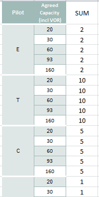
But I get the table as this:

etc etc..... How can i match fields in one excel sheet field to the other? Please help.

[sunny_talwar]

May be you need this

Sum(If(Pilot = Prod, Batch))