The Crosstable Load

[hic]

There are a number of prefixes in QlikView, that help you load and transform data. One of them is the Crosstable transformation.

[hic]

Whenever you have a crosstable of data, the Crosstable prefix can be used to transform the data and create the desired fields. A crosstable is basically a matrix where one of the fields is displayed vertically and another is displayed horizontally. In the input table below you have one column per month and one row per product.

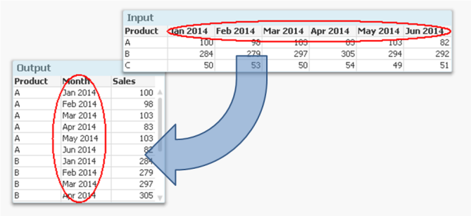
But if you want to analyze this data, it is much easier to have all numbers in one field and all months in another, i.e. in a three-column table. It is not very practical to have one column per month, since you want to use Month as dimension and Sum(Sales) as measure.

Enter the Crosstable prefix.

It converts the data to a table with one column for Month and another for Sales. Another way to express it is to say that it takes field names and converts these to field values. If you compare it to the Generic prefix, you will find that they in principle are each other’s inverses.

The syntax is

   Crosstable (Month, Sales) Load Product, [Jan 2014], [Feb 2014], [Mar 2014], … From … ;

There are however a couple of things worth noting:

• Usually the input data has only one column as qualifier field; as internal key (Product in the above example). But you can have several. If so, all qualifying fields must be listed before the attribute fields, and the third parameter to the Crosstable prefix must be used to define the number of qualifying fields.
• It is not possible to have a preceding Load or a prefix in front of the Crosstable keyword. Auto-concatenate will however work.
• The numeric interpretation will not work for the attribute fields. This means that if you have months as column headers, these will not be automatically interpreted. The work-around is to use the crosstable prefix to create a temporary table, and to run a second pass through it to make the interpretations:

   tmpData:

   Crosstable (MonthText, Sales)

   Load Product, [Jan 2014], [Feb 2014], … From Data;

   Final:

   Load Product,

      Date(Date#(MonthText,'MMM YYYY'),'MMM YYYY') as Month,

      Sales

      Resident tmpData;

   Drop Table tmpData;

Finally, if your source is a crosstable and you also want to display the data as a crosstable, it might be tempting to load the data as it is, without any transformation.

I strongly recommend that you don’t. A crosstable transformation simplifies everything and you can still display your data as a crosstable using a standard pivot table.

HIC

[valpassos]

Hi.

Any advice regarding this best practice question? stevedark‌, hic‌

Thanks!

[stevedark]

HI Lisa,

Glad you got the load working as required.

A good question about best practice.  As it stands, when the actual date rolls over, but the spreadsheet doesn't, you will be placing the wrong values in the wrong years. This is obviously a bad thing.

I would suggest that you put the year in the column heading, rather than Current and Previous etc..  That way you can just do a LOAD * from the spreadsheet and then have the right values appear in the right years. Adding a year is as simple as inserting a column and naming it correctly - if this doesn't happen on the 1st of Jan then it is not an issue.

Hope that makes sense?

[valpassos]

Hi Steve

Yes, that makes sense. But when the year 2019 rolls in, how exactly will the values be shifted?

I have this table now:

Sales:

CROSSTABLE (Year, Sales, 1)

LOAD

  Customer,

  "2018",

  "2017",

  "2016"

FROM Datasource;

;

But when the year 2019 rolls in, I will no longer need this table, right? How will I perform the incremental load just for the year 2019, maintaining the other years? stevedark‌

Thanks!

[stevedark]

Hi Lisa,

You could do an incremental for the new year, but what I would suggest makes more sense is inserting a new column to the left of 2018 and putting the 2019 figures there.  If you load with a wildcard then new columns will be picked up and dealt with automatically:

Sales:

CROSSTABLE (Year, Sales, 1)

LOAD

  *

FROM Datasource;

If you wanted to get subsequent years from another source it would just be a case of do your cross table as above then:

CONCATENATE(Sales)

LOAD

  Customer,

  2019 as Year,

  Sales

FROM NextYearDataSource;

Hope that makes sense?

Steve

[valpassos]

It makes perfect sense

Thanks, Steve!

[shalensookdeo]

Hi Henric Cronstrom

How would i load the following into qlikview. unfortunately my data is being pulled from sql and not excell but the columns are the same as per the screenshot below. Each column represents a month. How can pull the data into qlikview and then be able to select the month?

[robert99]

Hi Shalen

Have you tried the crosstable load?

This is an example I had to use for a similar situation

LOAD_BUDGET:

CrossTable (DateBudget,Budget,8)  // 8 equals the number of field to be loaded before the DateBudget

LOAD

RECNO() as RecNo,

[OC Entity],

    CIN#,

     [CIN Name],

    text (CSR#) as CSR#,

     [CSR Name] as CSR,

     text ([OC AR Nmbr]) as [OC AR Nmbr],

   etc ,

//2016 LOAD THE CROSSTABLE

"Net Posting 01" as 42370, // Jan 2016

    "Net Posting 02" as 42401,  // Feb 2016

    "Net Posting 03" as 42430, //march 2016

  etc

  FROM [lib://QADExcel/Database from the Cube Dec2016.xlsx]

(ooxml, embedded labels, table is Data);

This will laod

8 fields plus one field for the BudgetDate (from which a Month Year etc calendar can be created) and a final field for the amount.

[shalensookdeo]

Thank You, I will give it a try and revert.

Many Thanks

[alis2063]

nice explanation

[mg_gsi_da]

now I much better understand crosstables