Unlock a world of possibilities! Login now and discover the exclusive benefits awaiting you.
- Qlik Community
- :
- All Forums
- :
- Visualization and Usability
- :
- how to create a pie chart with 3 columns and count...
- Subscribe to RSS Feed
- Mark Topic as New
- Mark Topic as Read
- Float this Topic for Current User
- Bookmark
- Subscribe
- Mute
- Printer Friendly Page
- Mark as New
- Bookmark
- Subscribe
- Mute
- Subscribe to RSS Feed
- Permalink
- Report Inappropriate Content
how to create a pie chart with 3 columns and count the measures within the 3 columns
Dear all,
How do i create a pie chart with data (A, B, C) in different columns?
Field 1 | Field 2 | Field 3 |
| A | B | C |
| A | B | A |
| B | B | A |
the desired output is % of A, B and C in a pie chart. I was browsing around and could not understand and apply them to my scenario. Would appreciate if someone can assist.
A sample excel file is attached for your easy reference.
Thank you
Accepted Solutions
- Mark as New
- Bookmark
- Subscribe
- Mute
- Subscribe to RSS Feed
- Permalink
- Report Inappropriate Content
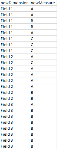
Is not possible for you in script change the load of the table and transpose in only 1 field?
In this case you can count only the field
Or you can use a formula like this
Dimension: =ValueList('A','B','C')
Measure:
if(ValueList('A','B','C')= 'A',Count({<[Field 1]={A}>}[Field 1]) + Count({<[Field 2]={A}>}[Field 2])+Count({<[Field 3]={A}>}[Field 3])
,
if(ValueList('A','B','C')= 'B',Count({<[Field 1]={B}>}[Field 1]) + Count({<[Field 2]={B}>}[Field 2])+Count({<[Field 3]={B}>}[Field 3])
,
if(ValueList('A','B','C')= 'C',Count({<[Field 1]={C}>}[Field 1]) + Count({<[Field 2]={C}>}[Field 2])+Count({<[Field 3]={C}>}[Field 3])
,
0
)
)
)
- Mark as New
- Bookmark
- Subscribe
- Mute
- Subscribe to RSS Feed
- Permalink
- Report Inappropriate Content
Hello Soh,
You need to do a CrossTable in the loading script to transform your 3 differents fields in 1.
From there, you can easily do a pie chart to get the % of A, B and C
- Mark as New
- Bookmark
- Subscribe
- Mute
- Subscribe to RSS Feed
- Permalink
- Report Inappropriate Content
Is not possible for you in script change the load of the table and transpose in only 1 field?
In this case you can count only the field
Or you can use a formula like this
Dimension: =ValueList('A','B','C')
Measure:
if(ValueList('A','B','C')= 'A',Count({<[Field 1]={A}>}[Field 1]) + Count({<[Field 2]={A}>}[Field 2])+Count({<[Field 3]={A}>}[Field 3])
,
if(ValueList('A','B','C')= 'B',Count({<[Field 1]={B}>}[Field 1]) + Count({<[Field 2]={B}>}[Field 2])+Count({<[Field 3]={B}>}[Field 3])
,
if(ValueList('A','B','C')= 'C',Count({<[Field 1]={C}>}[Field 1]) + Count({<[Field 2]={C}>}[Field 2])+Count({<[Field 3]={C}>}[Field 3])
,
0
)
)
)
- Mark as New
- Bookmark
- Subscribe
- Mute
- Subscribe to RSS Feed
- Permalink
- Report Inappropriate Content
the formula works for the earlier data set with 3 fields. So what happens if I have more than 3 fields or less than 3 fields? I tried this formula (amended from your version) for 2 fields (see attached excel) and my pie chart data is wrong. A should totalled 8, B = 4 and C = 4 but with the formula below, my pie chart shows A:16, B:8, B:8 .
| Field 1 | Field 2 |
| A | A |
| A | C |
| B | A |
| B | A |
| A | A |
| C | A |
| C | B |
| C | B |
if(ValueList('A','B','C')= 'A',Count({<[Field 1]={A}>}[Field 1]) + Count({<[Field 2]={A}>}[Field 2])
,
if(ValueList('A','B','C')= 'B',Count({<[Field 1]={B}>}[Field 1]) + Count({<[Field 2]={B}>}[Field 2])
,
if(ValueList('A','B','C')= 'C',Count({<[Field 1]={C}>}[Field 1]) + Count({<[Field 2]={C}>}[Field 2])
,
0
)
)
)
please advise what went wrong in the formula above. many thanks.
'Creating a CrossTable in the loading script to transform 3 differents fields in 1' is not preferred as the raw data consists of responses (20 questions & hence many columns of data) from a survey and I need the visualisation to tag the responses to the first few columns (student type, year of study & school). Many thanks for the idea still.
