Unlock a world of possibilities! Login now and discover the exclusive benefits awaiting you.
- Qlik Community
- :
- All Forums
- :
- QlikView App Dev
- :
- Re: Conditional formatting and comparison with the...
- Subscribe to RSS Feed
- Mark Topic as New
- Mark Topic as Read
- Float this Topic for Current User
- Bookmark
- Subscribe
- Mute
- Printer Friendly Page
- Mark as New
- Bookmark
- Subscribe
- Mute
- Subscribe to RSS Feed
- Permalink
- Report Inappropriate Content
Conditional formatting and comparison with the median value in the same pivot table
Hi everyone,
what I would like to do is to display in the same table the example you see in my excel attached in sheet "TO Display", you can see also the formulas.
I tried to do that in qvw but as you can see in my attached qvw, I'm stopped at the calculation of the % per Buyer/MonthYear.
Do you think that is possible to implement my excel example exactly in the same pivot table qvw?
Maybe I have to separate some of those information, average or median, in some other table?
Thanks for your help.
Filiberto
- « Previous Replies
-
- 1
- 2
- Next Replies »
Accepted Solutions
- Mark as New
- Bookmark
- Subscribe
- Mute
- Subscribe to RSS Feed
- Permalink
- Report Inappropriate Content
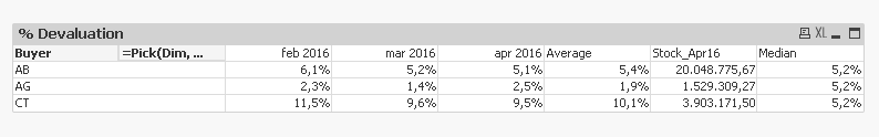
Maybe like this?
| Buyer | =Pick(Dim, MonthName(MonthYear), 'Average', 'Stock_Apr16', 'Median') | feb 2016 | mar 2016 | apr 2016 | Average | Stock_Apr16 | Median |
|---|---|---|---|---|---|---|---|
| AB | 6,1% | 5,2% | 5,1% | 5,5% | 20.048.775,67 | 5,5% | |
| AG | 2,3% | 1,4% | 2,5% | 2,1% | 1.529.309,27 | 5,5% | |
| CT | 11,5% | 9,6% | 9,5% | 10,2% | 3.903.171,50 | 5,5% |
You are calculating the average of averages in your excel file, while Sunny is calculating the expression total average (which I would personally prefer).
- Mark as New
- Bookmark
- Subscribe
- Mute
- Subscribe to RSS Feed
- Permalink
- Report Inappropriate Content
You can probably do this using a synthetic dimension, similar to what is shown here
Re: Show Pivot and Straight Table in One Table
I guess Sunny is already preparing a sample.
edit: this sample might be closer to your requirements:
- Mark as New
- Bookmark
- Subscribe
- Mute
- Subscribe to RSS Feed
- Permalink
- Report Inappropriate Content
This?
Script:
LOAD MonthYear,
Stock,
Devaluation,
Buyer
FROM
[Data.xlsx]
(ooxml, embedded labels);
Dim:
LOAD * Inline [
Dim
1
2
3
4];
Dimension:
Buyer
=Pick(Dim, MonthName(MonthYear), 'Average', 'Stock_Apr16', 'Median')
Expression
=Pick(Dim, Num(Sum(Devaluation)/Sum(Stock), '#.##0,0%'), Num(Sum(Devaluation)/Sum(Stock), '#.##0,0%'), Num(Sum({<MonthYear = {"$(=Max(MonthYear))"}>}Stock), '#.##0,00'), Num(Median(TOTAL Aggr(Sum(Devaluation)/Sum(Stock), Buyer, MonthYear)), '#.##0,0%'))
- Mark as New
- Bookmark
- Subscribe
- Mute
- Subscribe to RSS Feed
- Permalink
- Report Inappropriate Content
You are behind my samples 
- Mark as New
- Bookmark
- Subscribe
- Mute
- Subscribe to RSS Feed
- Permalink
- Report Inappropriate Content
stalwar1, you are still not writing blog on Pick
- Mark as New
- Bookmark
- Subscribe
- Mute
- Subscribe to RSS Feed
- Permalink
- Report Inappropriate Content
Hahahaha I am in the planning phase right now
- Mark as New
- Bookmark
- Subscribe
- Mute
- Subscribe to RSS Feed
- Permalink
- Report Inappropriate Content
Just implement, don't do any planning
- Mark as New
- Bookmark
- Subscribe
- Mute
- Subscribe to RSS Feed
- Permalink
- Report Inappropriate Content
That seems exactly as mine. But I can't understand 2 things:
1) the average is a little bit different from the value calculated in excel. What could be the reason?
2) The median value of the 3 values (2,1%; 5,5% ; 10,2%) must be 5,5%. Using the value of your example (1,9%; 5,4%; 10,1%) must be 5,4%. Not 5,2%. Don't you are agree?
- Mark as New
- Bookmark
- Subscribe
- Mute
- Subscribe to RSS Feed
- Permalink
- Report Inappropriate Content
1) Could be the rounding issue, not entirely sure what's wrong there
2) QlikView has it's own way to calculate Median, I think its doing it own weird calculation (I will have test it to be sure, but see this Re: What is the exactly calculation of the fractile function?)
- Mark as New
- Bookmark
- Subscribe
- Mute
- Subscribe to RSS Feed
- Permalink
- Report Inappropriate Content
Maybe like this?
| Buyer | =Pick(Dim, MonthName(MonthYear), 'Average', 'Stock_Apr16', 'Median') | feb 2016 | mar 2016 | apr 2016 | Average | Stock_Apr16 | Median |
|---|---|---|---|---|---|---|---|
| AB | 6,1% | 5,2% | 5,1% | 5,5% | 20.048.775,67 | 5,5% | |
| AG | 2,3% | 1,4% | 2,5% | 2,1% | 1.529.309,27 | 5,5% | |
| CT | 11,5% | 9,6% | 9,5% | 10,2% | 3.903.171,50 | 5,5% |
You are calculating the average of averages in your excel file, while Sunny is calculating the expression total average (which I would personally prefer).
- « Previous Replies
-
- 1
- 2
- Next Replies »