Field Issue

[vanderson009]

Hi Guys,

I have below data in my table,

Region	Type	Sales
North	Actual	456
East	Actual	348
South	Actual	123
West	Actual	487

I want to display it in pivot table as

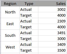
But my problem is, I have not Target Type in my Type column, I have only Actual Type, Can you please help me how can i achieve this scenario. 

Thanks and Regards,

Villyee.

[swuehl]

Where do the target values come from?

Do you have a different table with these values?

Or are these random numbers ?

[Chanty4u]

where that data coming from?

[vanderson009]

They are not coming from any table, I have to hard code that values,

that value are range value and i have to display it in Text formate.

On the basis of that range value i have to change background colour of actual value.

[vanderson009]

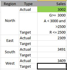
this is actual scenario, On the basis of Region, Range value will be different.

[swuehl]

Try a second expression labelled 'Target'

=Pick(

     Match(Region,'North','East','South','West'),    

                              4000, 4000,3000,3500)

[vanderson009]

Thanks swuehl...

I tried but because of second expression one more column is appeared in pivot table but i want row below actual type for every region.

[swuehl]

Have you tried pivoting your expressions columns to the left, so they appear as expression rows?

Pivot your columns by dragging the headers with the mouse.

[vanderson009]

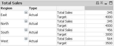
Yes i tried it but by dragging headers into row both expression are coming beside of actual type but i want target should appear below actual.

Attached is result

[swuehl]

Just rename the first expression from Total Sales to Actual, and remove dimension Type (it's a single value anyway).