Unlock a world of possibilities! Login now and discover the exclusive benefits awaiting you.
- Qlik Community
- :
- All Forums
- :
- QlikView App Dev
- :
- Help to create a profit and loss statement
- Subscribe to RSS Feed
- Mark Topic as New
- Mark Topic as Read
- Float this Topic for Current User
- Bookmark
- Subscribe
- Mute
- Printer Friendly Page
- Mark as New
- Bookmark
- Subscribe
- Mute
- Subscribe to RSS Feed
- Permalink
- Report Inappropriate Content
Help to create a profit and loss statement
Hi all,
I really need help with building a trend sheet with financial data and counts. This is a short version of what I would like to achieve:
| Category | |
| Paying customers | 10 |
| Free places | 2 |
| Total travellers | 12 |
| Group leaders | 1 |
| Tour revenue | 50,000.00 |
| Refunds | 2,000.00 |
| Discounts | 3,000.00 |
| Net tour revenue | 55,000.00 |
| Service revenue | 3,000.00 |
| Insurance revenue | 40,000.00 |
| Cancellation revenue | 5,500.00 |
| Total service revenue | 48,500.00 |
I attached a full version of what I would like to do, and the calculations I would do if I were about to calculate each number separately.
Can someone please help me out here and show me the smartest way to do this? Just let me know if you need further information in order to help me.
Thank you very much for your help and input 
Best,
Johanna
- Mark as New
- Bookmark
- Subscribe
- Mute
- Subscribe to RSS Feed
- Permalink
- Report Inappropriate Content
The way I have done this is to create a separate straight table for each line. Then supress the header rows of the straight tables on all excpet the top one. Then stack them one right after another so it looks like one table. This way to the user it looks like one table instead of multiple. As long as the time periods accross the top are the same for all of the categories on the left it won't be a problem. Two things to watch out for, obviously you can't use scrolling as there is no way to scroll all the charts at once. Make sure you uncheck allow move and size on the layout tab so no one accidentally moves them out of order.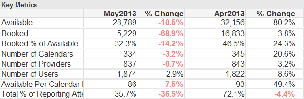
The end result would look like this...
- Mark as New
- Bookmark
- Subscribe
- Mute
- Subscribe to RSS Feed
- Permalink
- Report Inappropriate Content
Try the approach described in this document.
talk is cheap, supply exceeds demand
- Mark as New
- Bookmark
- Subscribe
- Mute
- Subscribe to RSS Feed
- Permalink
- Report Inappropriate Content
Can I still use IntervalMatch even though I already have a specific account grouping? How would you suggest to sort for this?