Unlock a world of possibilities! Login now and discover the exclusive benefits awaiting you.
- Qlik Community
- :
- All Forums
- :
- QlikView App Dev
- :
- Re: How to force null value into pivot table line
- Subscribe to RSS Feed
- Mark Topic as New
- Mark Topic as Read
- Float this Topic for Current User
- Bookmark
- Subscribe
- Mute
- Printer Friendly Page
- Mark as New
- Bookmark
- Subscribe
- Mute
- Subscribe to RSS Feed
- Permalink
- Report Inappropriate Content
How to force null value into pivot table line
Hi,
I'd like to ask a little help.
I have a pivot chart like this one below:
| Product | MeasureA | MeasureB |
|---|---|---|
A Product | 2 | 3 |
| B Product | 3 | 5 |
| C Product | 4 | 6 |
| Total | 9 | - |
MeasureA and MeasureB are sum(<set analysis>Volume) expressions.
I have to show null value in MeasureB column for total.
Does somebody know a working solution for this? I tried with Product -= {''Total'} in set analysis but it shows zero value in the total cell, but I need null value.
Thank you
Gabor
- « Previous Replies
-
- 1
- 2
- Next Replies »
Accepted Solutions
- Mark as New
- Bookmark
- Subscribe
- Mute
- Subscribe to RSS Feed
- Permalink
- Report Inappropriate Content
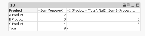
Try this expression:
=If(Product = 'Total', Null(), Sum({<Product -= {'Total'}>}MeasureB))
Output:
- Mark as New
- Bookmark
- Subscribe
- Mute
- Subscribe to RSS Feed
- Permalink
- Report Inappropriate Content
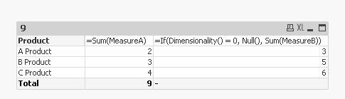
Try using the dimensionality() function for this:
If(Dimensionality() = 1, Null(), YourExpression)
If(Dimensionality() = 0, Null(), YourExpression)
- Mark as New
- Bookmark
- Subscribe
- Mute
- Subscribe to RSS Feed
- Permalink
- Report Inappropriate Content
Is total a row from the database or is a total you calculate in the chart?
- Mark as New
- Bookmark
- Subscribe
- Mute
- Subscribe to RSS Feed
- Permalink
- Report Inappropriate Content
This?
- Mark as New
- Bookmark
- Subscribe
- Mute
- Subscribe to RSS Feed
- Permalink
- Report Inappropriate Content
From the database. All of the Production columns value has dimensionality 1.
- Mark as New
- Bookmark
- Subscribe
- Mute
- Subscribe to RSS Feed
- Permalink
- Report Inappropriate Content
Total is an element from the Product. The dimensionality functions does not work in that case.
- Mark as New
- Bookmark
- Subscribe
- Mute
- Subscribe to RSS Feed
- Permalink
- Report Inappropriate Content
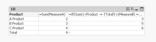
Try this expression:
=If(Sum({<Product -= {'Total'}>}MeasureB) = 0, Null(), Sum({<Product -= {'Total'}>}MeasureB)).
- Mark as New
- Bookmark
- Subscribe
- Mute
- Subscribe to RSS Feed
- Permalink
- Report Inappropriate Content
Thank you. The solution is closer, but it shows null instead of 0 if A Product = 0, but I need null only in the total row. Do you have an idea?
- Mark as New
- Bookmark
- Subscribe
- Mute
- Subscribe to RSS Feed
- Permalink
- Report Inappropriate Content
Try this expression:
=If(Product = 'Total', Null(), Sum({<Product -= {'Total'}>}MeasureB))
Output:
- Mark as New
- Bookmark
- Subscribe
- Mute
- Subscribe to RSS Feed
- Permalink
- Report Inappropriate Content
Perfect! Thank you!
- « Previous Replies
-
- 1
- 2
- Next Replies »