Unlock a world of possibilities! Login now and discover the exclusive benefits awaiting you.
- Qlik Community
- :
- All Forums
- :
- QlikView App Dev
- :
- Pivot Table calculated Dimension not applying filt...
- Subscribe to RSS Feed
- Mark Topic as New
- Mark Topic as Read
- Float this Topic for Current User
- Bookmark
- Subscribe
- Mute
- Printer Friendly Page
- Mark as New
- Bookmark
- Subscribe
- Mute
- Subscribe to RSS Feed
- Permalink
- Report Inappropriate Content
Pivot Table calculated Dimension not applying filter of other dimensions
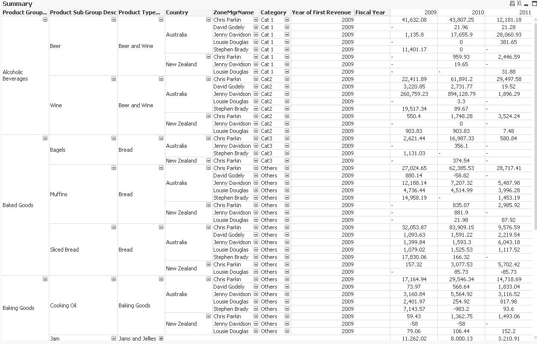
I have a Pivot Table.

The column 'Year of first Revenue' is a Calculated Dimension with this formula
=IF($(=Sum({<[Fiscal Year]={$(=(vCurrentYear)-2)}>}[Sales Amount])) = 0, 'None', $(=(vCurrentYear)-2))
The result in column Year of First Revenue is not applied the filters of other dimensions, namely Product Group des, Product Sub Group Desc etc... In other words, (=Sum({<[Fiscal Year]={$(=(vCurrentYear)-2)}>}[Sales Amount])) is the sum of all sales for 2009 for all Product Group Desc, Product Sub Group Desc etc...
I would like the value for the dimension Year of first Revenue to be the sum of Sales Amount for each individual cell in the Pivot Table.
Is there a way to implement this ?
Regards