Unlock a world of possibilities! Login now and discover the exclusive benefits awaiting you.
- Qlik Community
- :
- All Forums
- :
- QlikView App Dev
- :
- Sort Order
- Subscribe to RSS Feed
- Mark Topic as New
- Mark Topic as Read
- Float this Topic for Current User
- Bookmark
- Subscribe
- Mute
- Printer Friendly Page
- Mark as New
- Bookmark
- Subscribe
- Mute
- Subscribe to RSS Feed
- Permalink
- Report Inappropriate Content
Sort Order
Hi Friends
I have following Pivot table in my doc
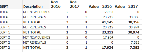
I want to Total Column come to the bottom of table and Dept 1 & Dept 2 to remain as it is. The sorting order is
sum(PREMIUM) descending
Further I have a calculated dimension as shown below
=pick(Dim,DEPT,'TOTAL')
Pls help me
- « Previous Replies
-
- 1
- 2
- Next Replies »
Accepted Solutions
- Mark as New
- Bookmark
- Subscribe
- Mute
- Subscribe to RSS Feed
- Permalink
- Report Inappropriate Content
Check with this
RangeSum(Only({1} DimF), -sum({<RISK_YEAR = {$(=Max(RISK_YEAR))},RISK_DATE={$(vP17)}>}PREMIUM)/1e10)
- Mark as New
- Bookmark
- Subscribe
- Mute
- Subscribe to RSS Feed
- Permalink
- Report Inappropriate Content
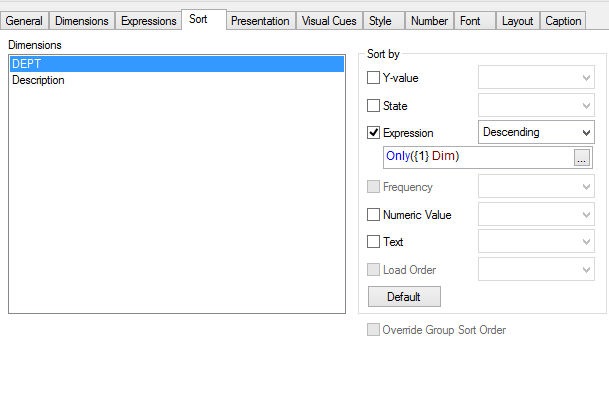
Sort this dimension using this expression:
Only({1} Dim)
- Mark as New
- Bookmark
- Subscribe
- Mute
- Subscribe to RSS Feed
- Permalink
- Report Inappropriate Content
still no change Same result
- Mark as New
- Bookmark
- Subscribe
- Mute
- Subscribe to RSS Feed
- Permalink
- Report Inappropriate Content
Did you sort this calculated dimension (=pick(Dim,DEPT,'TOTAL')) using this -> (Only({1} Dim)) on the sort tab?
- Mark as New
- Bookmark
- Subscribe
- Mute
- Subscribe to RSS Feed
- Permalink
- Report Inappropriate Content
Yes Sunny
- Mark as New
- Bookmark
- Subscribe
- Mute
- Subscribe to RSS Feed
- Permalink
- Report Inappropriate Content
Change Descending to Ascending.
Also mark the Text checkbox and see if it works.
Regards,
Kaushik Solanki
- Mark as New
- Bookmark
- Subscribe
- Mute
- Subscribe to RSS Feed
- Permalink
- Report Inappropriate Content
Then Total comes in between Dept
- Mark as New
- Bookmark
- Subscribe
- Mute
- Subscribe to RSS Feed
- Permalink
- Report Inappropriate Content
Uncheck the sorting order for Description and check.
If that also doesnt work then please share the sample data to understand it in detail.
Regards,
Kaushik Solanki
- Mark as New
- Bookmark
- Subscribe
- Mute
- Subscribe to RSS Feed
- Permalink
- Report Inappropriate Content
Try this
RangeSum(Only({1} Dim), Rank(DEPT))
and sort ascending
If that doesn't work, try this
RangeSum(Only({1} Dim), -Rank(DEPT))
and sort ascending
- Mark as New
- Bookmark
- Subscribe
- Mute
- Subscribe to RSS Feed
- Permalink
- Report Inappropriate Content
I have tried that but still not working. I have attached my sample data pls advise
- « Previous Replies
-
- 1
- 2
- Next Replies »