Totals Row with Specific Values

[Anonymous]

Hello.  I am wondering if there is a way to create a separate totals row in addition to the grand totals row in a pivot table.  For example, if I have the table below, here is what I am trying to do:

M&M's

Red         6

Green     4

Blue        2

Yellow    5

===========

Red and Blue subtotal   8

Grand Total  17

How do I create the conditional subtotal?  Thank you

[jpenuliar]

Hi Robert,

Try and make use of Dimensionality() function.

Example in expression :

=If(Dimensionality() = 0

    ,Sum({<Colour = {'Red','Blue'}>}[M&M]) & chr(13) & Sum([M&M])

    ,Sum([M&M])

)

should look like below:

[jpenuliar]

Label for Totals:

=If(Dimensionality() = 0

    ,'Red and Blue subtotal' & chr(13)& 'Grand Total' 

)

[Anonymous]

What if the values are calculated?  For example, if the value for blue M&M's is actually created using a formula and not a straight value from the table?

[jpenuliar]

hmmm, I suppose the logic should be Red & Blue = exressionRed + expressionBlue.

Can you post a sample data/app?

[Anonymous]

Jonathan I have tried your suggestions (modifying my data for security purposes and creating a view of straight data) and so far have a table that looks like this:

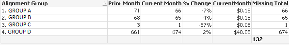
I used this code to create the table above:

=If(Dimensionality() = 0,Sum({<grp_typ = {'1. GROUP A','2. GROUP B','3. GROUP C'}>}[Current Month]) & chr(13) & Sum([Current Month]),Sum([Current Month]))

and this for the label:

=If(Dimensionality() = 0,'Missing Total' & chr(13)& 'Grand Total')

what am I doing wrong?  I am trying to make my table look like this:

[jpenuliar · Accepted solution]

You probably need to tick MultiLine Setting> adjust Wrap Cell Height to show the next line created by chr(13)

[Anonymous]

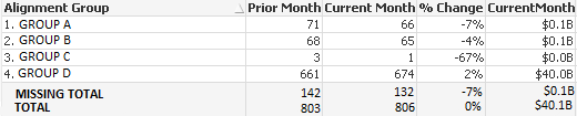
OK Jonathan I am much closer now.  Here's my table:

I am trying to figure out why my percentage totals are so far off now.  Thank you for your help