how to show 3 expression column's in Single row in Pivot table ?

[#1]

Hi i have pivot table below is the actual format

Region	Red	amber	green
India	1	4	6
Delhi	3	9	0

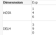
Output:

Region	Exp
India	1 4 6
Delhi	3 9 0

i want above output in Pivot table please help

[yoganantha321]

hi chaganti,

Kindly use cross table to get the status field and use it in pivot table.

Example:

I have 3 field tax,aadhar,passport each status in one field

crosstable (Document,Status)

LOAD EmployeeID,

TaxIDStatus as TaxID,

     AadharIDStatus as AadharID,

     PassportStatus as Passport,

Resident Employee_Info;

the table will be look like below:

the data will be

the status field can be called in pivot table

I think this will be useful

[hector_munoz]

Hi Chaganti,

What is the desired output? First or second one? Could you attach a sample?

Regards,

H

[#4]

updated please check

[hector_munoz]

Hi Chaganti, could you send us the formula of each expression?

[#6]

simple expressioons

Sum(Red) ,Sum(green), Sum(Amber) and Country dimension

[Anil_Babu_Samineni]

Create Pivot Table and use expression as

Sum(Red) & Chr(10) & Sum(amber) & chr(10) & Sum(green)

[#8]

its not working its only diplaying sum(Red) remaing not showing

[Anil_Babu_Samineni]

Strange, I have done and it's working. Go to presentation and extend cell height and then check