Unlock a world of possibilities! Login now and discover the exclusive benefits awaiting you.
- Qlik Community
- :
- All Forums
- :
- QlikView App Dev
- :
- Re: pivot dimension background color without expre...
- Subscribe to RSS Feed
- Mark Topic as New
- Mark Topic as Read
- Float this Topic for Current User
- Bookmark
- Subscribe
- Mute
- Printer Friendly Page
- Mark as New
- Bookmark
- Subscribe
- Mute
- Subscribe to RSS Feed
- Permalink
- Report Inappropriate Content
pivot dimension background color without expression
Dear Community,
we noticed that if we use a pivot without an expression, we can not set the background color of dimensions.
Is there any possibility how to achive that?
We need the pivot as it groups fields, but we dont have an expression. Maybe hiding an dummy expression would be a solution?
Accepted Solutions
- Mark as New
- Bookmark
- Subscribe
- Mute
- Subscribe to RSS Feed
- Permalink
- Report Inappropriate Content
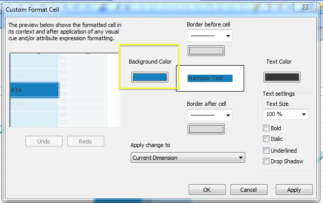
first go to settings>document properties>general and check that styling mode is set to advanced.
now right click on pivot table > select custom format cell>click on background colour and choose colour
hope this works
- Mark as New
- Bookmark
- Subscribe
- Mute
- Subscribe to RSS Feed
- Permalink
- Report Inappropriate Content
see this,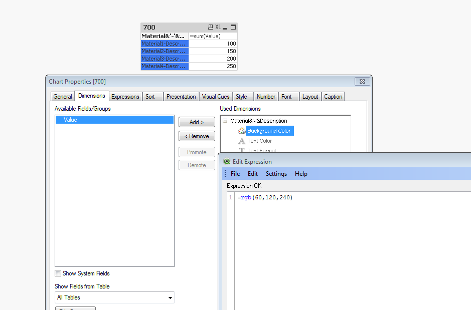
- Mark as New
- Bookmark
- Subscribe
- Mute
- Subscribe to RSS Feed
- Permalink
- Report Inappropriate Content
Hi Shiva, your example has a expression, thats what we dont want!
- Mark as New
- Bookmark
- Subscribe
- Mute
- Subscribe to RSS Feed
- Permalink
- Report Inappropriate Content
Hi Sana, your answer is correct, you just forgot to mention that we have to active "Design Grid.
Thanks!
- Mark as New
- Bookmark
- Subscribe
- Mute
- Subscribe to RSS Feed
- Permalink
- Report Inappropriate Content
ur right,but the background color is applied only for dimensions objects..so u can do the same on ur pivot table whether ur have expression or even if u don't ve expression.
- Mark as New
- Bookmark
- Subscribe
- Mute
- Subscribe to RSS Feed
- Permalink
- Report Inappropriate Content
Thats the point if you dont have an expression it will not work... 
Then you have to use "custom format cell", which was mentioned by Sana.
- Mark as New
- Bookmark
- Subscribe
- Mute
- Subscribe to RSS Feed
- Permalink
- Report Inappropriate Content
ya,even tht's other option..i never tried with out expression..so i thought it'll works 
- Mark as New
- Bookmark
- Subscribe
- Mute
- Subscribe to RSS Feed
- Permalink
- Report Inappropriate Content
If we now use an expression for the background color (matching value of row) of the custom format cell, and the expression matches a value in one row, all rows get colored.
Is there any way how we can achive this, that only the row with the matched value gets colored while using custom format cell with an expression?
- Mark as New
- Bookmark
- Subscribe
- Mute
- Subscribe to RSS Feed
- Permalink
- Report Inappropriate Content
Custom Format cell only used to color the Header fields only (Table Field Name BG)