Unlock a world of possibilities! Login now and discover the exclusive benefits awaiting you.
- Qlik Community
- :
- All Forums
- :
- QlikView App Dev
- :
- Re: pivot table - getting expressions horizantal i...
- Subscribe to RSS Feed
- Mark Topic as New
- Mark Topic as Read
- Float this Topic for Current User
- Bookmark
- Subscribe
- Mute
- Printer Friendly Page
- Mark as New
- Bookmark
- Subscribe
- Mute
- Subscribe to RSS Feed
- Permalink
- Report Inappropriate Content
pivot table - getting expressions horizantal instead of vertical
Hi all,
Hope you are all well. I am trying to do a pivot table. Dimensions are: Dept Code, Result, Target and Month. The expression is sum(OrderActual).
I can pivot things but the result I am trying to get is attached in the excel spreadsheet (End Result) and also pasted below.
I tried to add calculated dimension with the formula =sum({<Result={'AB'}>}OrderActual)/sum({<Result={'OPSRIC'}>}OrderActual), I get an error message.
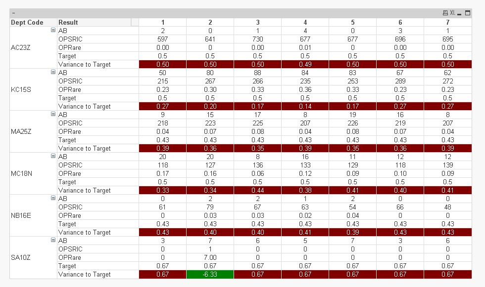
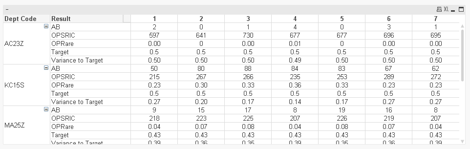
As you can see below, I am trying to get AB, OPSPRIC, OPRate (which will be the result of the above expression), Target, and Variance TO Target (which would be 'Target-OPRate') - ALL HORIZANTALY just like below. In Background colour, I would like to say, IF(Target-OPRate)>0, Red, Green). Any help is appreciated.
| Dept Code | Result | Month | At Month 6 | |||||
| 1 | 2 | 3 | 4 | 5 | 6 | |||
| AC23Z | AB | 2 | 0 | 1 | 4 | 0 | 3 | 10 |
| OPSRIC | 597 | 641 | 730 | 677 | 677 | 695 | 4017 | |
| OPRate | 0.00 | 0.00 | 0.00 | 0.01 | 0.00 | 0.00 | 0.00 | |
| Target | 0.05 | 0.05 | 0.05 | 0.05 | 0.05 | 0.05 | 0.05 | |
| variance to Target | -0.047 | -0.050 | -0.049 | -0.044 | -0.050 | -0.046 | -0.048 | |
| KC15S | AB | 40 | 68 | 71 | 62 | 72 | 48 | 361 |
| OPSRIC | 148 | 195 | 194 | 162 | 199 | 218 | 1116 | |
| OPRate | 0.27 | 0.35 | 0.37 | 0.38 | 0.36 | 0.22 | 0.32 | |
| Target | 0.05 | 0.05 | 0.05 | 0.05 | 0.05 | 0.05 | 0.05 | |
| variance to Target | 0.220 | 0.299 | 0.316 | 0.333 | 0.312 | 0.170 | 0.273 | |
Thanks,
Karthik
Accepted Solutions
- Mark as New
- Bookmark
- Subscribe
- Mute
- Subscribe to RSS Feed
- Permalink
- Report Inappropriate Content
This?
Background color expression
If(Dim = 4,
If(Sum({<Result={'AB'}>}OrderActual)/sum({<Result={'OPSRIC'}>}OrderActual) > Target, Green(), Red()))
- Mark as New
- Bookmark
- Subscribe
- Mute
- Subscribe to RSS Feed
- Permalink
- Report Inappropriate Content
Is this what you want?
- Mark as New
- Bookmark
- Subscribe
- Mute
- Subscribe to RSS Feed
- Permalink
- Report Inappropriate Content
Hi Sunil,
exactly what what I wanted. I will look at it when I reach home. Thank you very much. I don't have Qlikview server access. I will give it a go and let you know.
- Mark as New
- Bookmark
- Subscribe
- Mute
- Subscribe to RSS Feed
- Permalink
- Report Inappropriate Content
Sounds like a plan. Btw my name is Sunny (not Sunil) my friend 
- Mark as New
- Bookmark
- Subscribe
- Mute
- Subscribe to RSS Feed
- Permalink
- Report Inappropriate Content
oops, sorry Sunny! I think it was the auto text!
- Mark as New
- Bookmark
- Subscribe
- Mute
- Subscribe to RSS Feed
- Permalink
- Report Inappropriate Content
no problem
- Mark as New
- Bookmark
- Subscribe
- Mute
- Subscribe to RSS Feed
- Permalink
- Report Inappropriate Content
Hi Sunny,
Thanks again for the response and it is working great! However, I tried to colour code the 'Variance to Target' row. In principle, if Target > OPRare, it should be red, otherwise green. I tried various combinations that you have used under 'Expressions' but I am doing something wrong. The closest I could get to (still not correct) is with the below, but it highlights the OPRare and the Target field rather than the 'Variance to Target' field. Clearly, I am doing something wrong. Please could you point me in the right direction.
=PICK(Dim, Num(Sum({<POD={'DC'}>}ActivityActual)/sum({<POD={'OPPROC'}>}ActivityActual), '##.00')>Target, Green(), Red())
Thanks,
Karthik
- Mark as New
- Bookmark
- Subscribe
- Mute
- Subscribe to RSS Feed
- Permalink
- Report Inappropriate Content
This?
Background color expression
If(Dim = 4,
If(Sum({<Result={'AB'}>}OrderActual)/sum({<Result={'OPSRIC'}>}OrderActual) > Target, Green(), Red()))
- Mark as New
- Bookmark
- Subscribe
- Mute
- Subscribe to RSS Feed
- Permalink
- Report Inappropriate Content
That is it!! Thank you very much Sunny, extremely helpful.