Unlock a world of possibilities! Login now and discover the exclusive benefits awaiting you.
- Qlik Community
- :
- All Forums
- :
- QlikView
- :
- Changing color for individual column header in a s...
- Subscribe to RSS Feed
- Mark Topic as New
- Mark Topic as Read
- Float this Topic for Current User
- Bookmark
- Subscribe
- Mute
- Printer Friendly Page
- Mark as New
- Bookmark
- Subscribe
- Mute
- Subscribe to RSS Feed
- Permalink
- Report Inappropriate Content
Changing color for individual column header in a straight table
Hi.
If you need customise labels in a straight table and for some reasons you can't use pivot table, I have prepared this little trick. This solution is not very friendly and have few limitations but maybe it will inspire someone to prepare better solution.

How can you achieve such an effect?
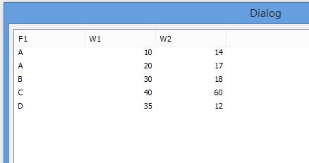
Source table:
1. Adding dimension to a Straight table
=ValueList($(=Chr(39) & concat( F1, Chr(39) & ',' & chr(39)) & Chr(39)),'Label')
We use values from field F1 and add value 'Label' for name of dimension
To use function ValueList we have to concat values from field F1.
I have used this trick from this topic. @https://community.qlik.com/thread/135024
Thanks RubenMarin
2. In first expression we can use this logic
IF(ValueList($(=Chr(39) & concat( F1, Chr(39) & ',' & chr(39)) & Chr(39)),'Label')='Label','Column 1',

SUM(If(F1=ValueList($(=Chr(39) & concat( F1, Chr(39) & ',' & chr(39)) & Chr(39)),'Label'),W1)))
If dimension is equal to our added value, we can put name of our label for this expression.
In above expression I sum other values.
3. In Presentation tab we check 'supress header row'
4. In Sort tab in first dimension we use 'Load order - Reversed'
5. Finally, we can customise our labels in first row.
For example if we want to change background, we can change it in expression properties:
=if(ValueList($(=Chr(39) & concat( F1, Chr(39) & ',' & chr(39)) & Chr(39)),'Label')='Label',Yellow(),10)
Thanks to KatarzynaScibor for support
- Tags:
- color formate
- labels
- qlikview visualization
- qlikview_layout_visualizations
- straight table
- visuliazation
- Mark as New
- Bookmark
- Subscribe
- Mute
- Subscribe to RSS Feed
- Permalink
- Report Inappropriate Content
Thanks Piotr for this case!