Unlock a world of possibilities! Login now and discover the exclusive benefits awaiting you.
- Qlik Community
- :
- All Forums
- :
- QlikView App Dev
- :
- Combining Pivot Tables into one table
- Subscribe to RSS Feed
- Mark Topic as New
- Mark Topic as Read
- Float this Topic for Current User
- Bookmark
- Subscribe
- Mute
- Printer Friendly Page
- Mark as New
- Bookmark
- Subscribe
- Mute
- Subscribe to RSS Feed
- Permalink
- Report Inappropriate Content
Combining Pivot Tables into one table
Hi,
Now you're probably thinking I should have used the search function. I did, but unfortunately can't find my exact problem with a solution, so here goes 
If I have a table like so:
| Name | Colour | Job | City | Date |
| 1 | G | Driver | London | 01/01/2016 |
| 2 | R | Walker | Paris | 02/01/2016 |
| 3 | B | Swimmer | Paris | 01/05/2016 |
| 4 | R | Swimmer | NY | 03/06/2016 |
| 5 | G | Driver | Dakar | 17/06/2016 |
| 6 | B | Sleeper | Timbuktu | 02/12/2017 |
I can create Pivot tables that look like:
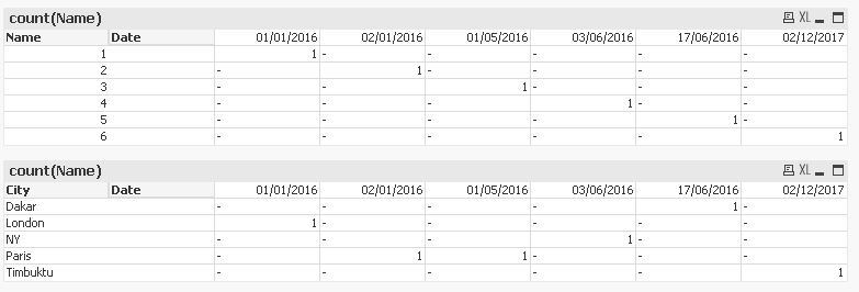
I would like to be able to combine those tables so that the caption and Date line don't appear on the second table and the City lines appear directly below the Name lines, like an Excel KPI based on 'Date' would look like. ie:

Many Thanks
Accepted Solutions
- Mark as New
- Bookmark
- Subscribe
- Mute
- Subscribe to RSS Feed
- Permalink
- Report Inappropriate Content
- Mark as New
- Bookmark
- Subscribe
- Mute
- Subscribe to RSS Feed
- Permalink
- Report Inappropriate Content
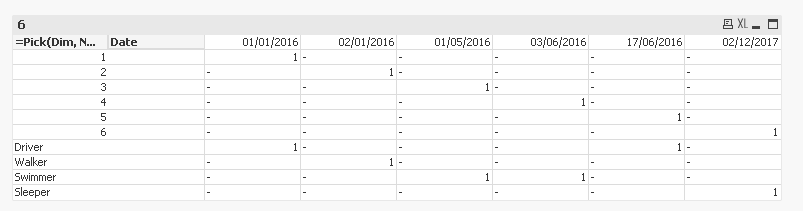
Like this?
- Mark as New
- Bookmark
- Subscribe
- Mute
- Subscribe to RSS Feed
- Permalink
- Report Inappropriate Content
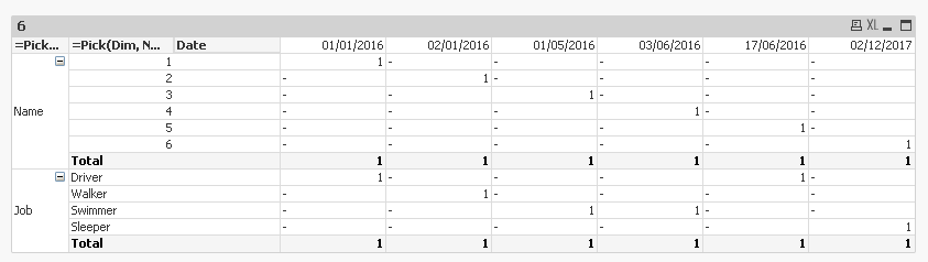
Hi Sunny,
That is very very useful thank you, but is there a way to keep the name of the dimension inbetween the rows, and also a way to show the subtotals of each date?
- Mark as New
- Bookmark
- Subscribe
- Mute
- Subscribe to RSS Feed
- Permalink
- Report Inappropriate Content
How about something like this?
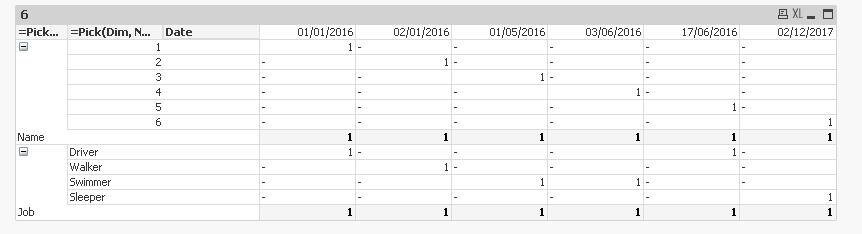
Or this
- Mark as New
- Bookmark
- Subscribe
- Mute
- Subscribe to RSS Feed
- Permalink
- Report Inappropriate Content
Perfect, many many thanks. Now researching the 'pick' function 