Unlock a world of possibilities! Login now and discover the exclusive benefits awaiting you.
- Qlik Community
- :
- All Forums
- :
- Qlik NPrinting
- :
- Excel conditional formatting lost when using nprin...
- Subscribe to RSS Feed
- Mark Topic as New
- Mark Topic as Read
- Float this Topic for Current User
- Bookmark
- Subscribe
- Mute
- Printer Friendly Page
- Mark as New
- Bookmark
- Subscribe
- Mute
- Subscribe to RSS Feed
- Permalink
- Report Inappropriate Content
Excel conditional formatting lost when using nprinting 17 levels
Am generating an excel file using nprinting 17. I conditionally format a couple of cells, within in a table(that i created using columns from a qliksense object in the excel template) such that if the value in one cell is greater than the other cell, its shaded green or else red. It was working fine.
The moment i introduced a level and then wrapped it around the previously created table - the level functionality was working fine as it was spanning out tables in the same worksheet for the various values of the level that I added. However, the conditional formatting was totally last. I can no longer see the cells shaded as per the conditional formatting rule that I set up earlier.
Is this a known issue or am i missing something here ? Help.
- « Previous Replies
-
- 1
- 2
- Next Replies »
Accepted Solutions
- Mark as New
- Bookmark
- Subscribe
- Mute
- Subscribe to RSS Feed
- Permalink
- Report Inappropriate Content
Hi,
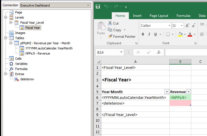
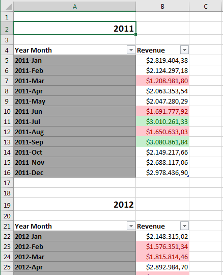
I suggest you to apply the Excel conditional formatting to two rows (the green and the red ones in the picture) in the template. Then add a <deleterow> tag at the beginning of the unuseful row so it will be deleted from the produced report.
Best Regards,
Ruggero
---------------------------------------------
When applicable please mark the appropriate replies as CORRECT. This will help community members and Qlik Employees know which discussions have already been addressed and have a possible known solution. Please mark threads as HELPFUL if the provided solution is helpful to the problem, but does not necessarily solve the indicated problem. You can mark multiple threads as HELPFUL if you feel additional info is useful to others.
Best Regards,
Ruggero
---------------------------------------------
When applicable please mark the appropriate replies as CORRECT. This will help community members and Qlik Employees know which discussions have already been addressed and have a possible known solution. Please mark threads with a LIKE if the provided solution is helpful to the problem, but does not necessarily solve the indicated problem. You can mark multiple threads with LIKEs if you feel additional info is useful to others.
- Mark as New
- Bookmark
- Subscribe
- Mute
- Subscribe to RSS Feed
- Permalink
- Report Inappropriate Content
Do you have an example of the excel formula and the table you can share so we can have a look please.
- Mark as New
- Bookmark
- Subscribe
- Mute
- Subscribe to RSS Feed
- Permalink
- Report Inappropriate Content
Hi Darrell,
Attached screenshots of the excel that i am using and the formula that is relevant.
When I don't include the <RMLevel>, the table prints out fine and the colors look correct. The moment I pull the <RMLevel> to the template, the level works fine, as in the table you see is repeated for each of the values of the RMLevel - but the color coding is totally missing.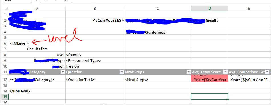
- Mark as New
- Bookmark
- Subscribe
- Mute
- Subscribe to RSS Feed
- Permalink
- Report Inappropriate Content
Have you tried defining your table and referencing that in your formula rather than cells. The issue will be the level moves the cell start for each table instance. by defining and referencing your table it should hold the formatting.
- Mark as New
- Bookmark
- Subscribe
- Mute
- Subscribe to RSS Feed
- Permalink
- Report Inappropriate Content
Hey Andy,
Not completely sure what you meant there when you say "Defining your table". The table that you see in my screenshot is straight out of qliksense. I added it to the tables node in excel and then dragged each of the table columns manually into the excel template.
didn't really get the "Defining and referencing your table" either. Can you explain a bit please.
- Mark as New
- Bookmark
- Subscribe
- Mute
- Subscribe to RSS Feed
- Permalink
- Report Inappropriate Content
You can highlight your table area and give it a name for reference. I've used it to identify the data source for pivot tables using nprinting.
I'll have a go at it tomorrow morning and get an example working as it should work.
- Mark as New
- Bookmark
- Subscribe
- Mute
- Subscribe to RSS Feed
- Permalink
- Report Inappropriate Content
ok.Thanks.
But am interested in formatting only one of the columns in the table ! Should I be referencing a table ?
- Mark as New
- Bookmark
- Subscribe
- Mute
- Subscribe to RSS Feed
- Permalink
- Report Inappropriate Content
Andy,
just some more detail.
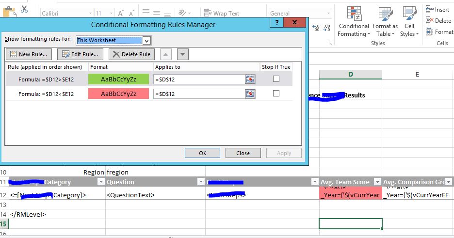
My goal is to repeat the table that you're seeing for each value of the RMLevel. So am nesting the table within the RMLevel tags- After which I expect to something like this as in the attached image here. I expect to see only the Avg.Team Score column shaded in either red/green in comparison with the avg.comparison group score on the right.
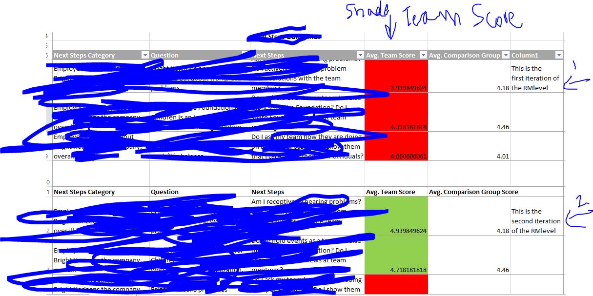
Also, I am creating a page for each category, so the above table is repeated across worksheets also, for each value of the page-fyi. Anyways, if we can make it work for one sheet-it should work for all the pages as well. thanks !
- Mark as New
- Bookmark
- Subscribe
- Mute
- Subscribe to RSS Feed
- Permalink
- Report Inappropriate Content
Hi,
I suggest you to apply the Excel conditional formatting to two rows (the green and the red ones in the picture) in the template. Then add a <deleterow> tag at the beginning of the unuseful row so it will be deleted from the produced report.
Best Regards,
Ruggero
---------------------------------------------
When applicable please mark the appropriate replies as CORRECT. This will help community members and Qlik Employees know which discussions have already been addressed and have a possible known solution. Please mark threads as HELPFUL if the provided solution is helpful to the problem, but does not necessarily solve the indicated problem. You can mark multiple threads as HELPFUL if you feel additional info is useful to others.
Best Regards,
Ruggero
---------------------------------------------
When applicable please mark the appropriate replies as CORRECT. This will help community members and Qlik Employees know which discussions have already been addressed and have a possible known solution. Please mark threads with a LIKE if the provided solution is helpful to the problem, but does not necessarily solve the indicated problem. You can mark multiple threads with LIKEs if you feel additional info is useful to others.
- Mark as New
- Bookmark
- Subscribe
- Mute
- Subscribe to RSS Feed
- Permalink
- Report Inappropriate Content
Have you tried just adding the tags in row 11 and 12 without the excel table function. Do you really need this data in an excel table?
I have a similar report I have built that uses conditional formatting in a table (BUT NOT USING EXCEL TABLE JUST TAGS IN CELLS) just like yours and the formatting works OK.
- « Previous Replies
-
- 1
- 2
- Next Replies »