Unlock a world of possibilities! Login now and discover the exclusive benefits awaiting you.
- Qlik Community
- :
- All Forums
- :
- QlikView App Dev
- :
- Bar chart display
- Subscribe to RSS Feed
- Mark Topic as New
- Mark Topic as Read
- Float this Topic for Current User
- Bookmark
- Subscribe
- Mute
- Printer Friendly Page
- Mark as New
- Bookmark
- Subscribe
- Mute
- Subscribe to RSS Feed
- Permalink
- Report Inappropriate Content
Bar chart display
Hi Team,
I have column called CAL_Period. The data in the column is of the of format 'YYYYMM'
The starting value is 199305, End value is 201612.
Question:
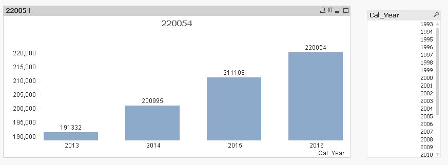
I need to show 4 bars in bar chart. 1st bar current year, 2nd for current year -1, 3rd for current year-2, 4th for current year -3. These bars should display from right to left.
That is , 2013, 2014, 2015, 2016
for 2013 bar, i need to show the sum of my measure starting from 199305 to 201312
for 2014 bar, i need to show from 199305 to 201412
for 2015 bar, i need to show from 199305 to 201512
for 2016 bar, i need to show from 199305 to 201612
How to implement this.
Regards
Srinivas
- « Previous Replies
-
- 1
- 2
- Next Replies »
Accepted Solutions
- Mark as New
- Bookmark
- Subscribe
- Mute
- Subscribe to RSS Feed
- Permalink
- Report Inappropriate Content
For year, you can try this:
=RangeSum(Above(Sum({<Cal_Period, Cal_Year>}Sales), 0, RowNo())) * Avg({<Cal_Year = {"$(='>=' & (Max(Cal_Year)-3) & '<=' & Max(Cal_Year))"}>}1)
- Mark as New
- Bookmark
- Subscribe
- Mute
- Subscribe to RSS Feed
- Permalink
- Report Inappropriate Content
Have you read these thread my friend?
QlikCommunity Tip: How to get answers to your post?
Preparing examples for Upload - Reduction and Data Scrambling
We are all trying to help each other, but you need to give us enough information so that we can help you as quickly as possible 
- Mark as New
- Bookmark
- Subscribe
- Mute
- Subscribe to RSS Feed
- Permalink
- Report Inappropriate Content
Hi,
You should have year field in your data, use that year field as your dimension and select Full accumulation in Expression tab.
If your calendar is properly mapped, You will get your desired results,
Regards,
Ganesh
- Mark as New
- Bookmark
- Subscribe
- Mute
- Subscribe to RSS Feed
- Permalink
- Report Inappropriate Content
Attached the sample data
Regards
Srinivas
- Mark as New
- Bookmark
- Subscribe
- Mute
- Subscribe to RSS Feed
- Permalink
- Report Inappropriate Content
I have cal_Year column. This column i am using as dimension.
I have issue in creating the expression.
Regards
Srinivas
- Mark as New
- Bookmark
- Subscribe
- Mute
- Subscribe to RSS Feed
- Permalink
- Report Inappropriate Content
the easy solution :
create 4 expressions as follows :
Sum({<Cal_Period={"<=201312"}>} Sales)
Sum({<Cal_Period={"<=201412"}>} Sales)
Sum({<Cal_Period={"<=201512"}>} Sales)
Sum({<Cal_Period={"<=201612"}>} Sales)
- Mark as New
- Bookmark
- Subscribe
- Mute
- Subscribe to RSS Feed
- Permalink
- Report Inappropriate Content
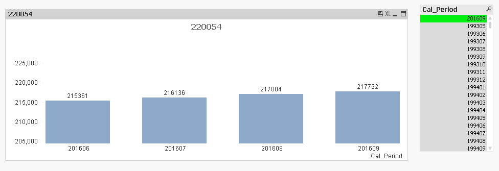
May be this:
=RangeSum(Above(Sum({<Cal_Period>}Sales), 0, RowNo())) * Avg({<Cal_Period = {"$(='>=' & Date(AddMonths(Max(Cal_Period), -3), 'YYYYMM') & '<=' & Date(AddMonths(Max(Cal_Period), 0), 'YYYYMM'))"}>}1)
- Mark as New
- Bookmark
- Subscribe
- Mute
- Subscribe to RSS Feed
- Permalink
- Report Inappropriate Content
You are right and it should bring the values as expected.
But, when i take CAL_Year as my dimension, it is showing the bars for 2011, 2012 also,
I need to show only 2013, 2014,2015 and 2016 values related bars.
Is there any other way to restrict the year based on the expression?
Regards
Srinivas
- Mark as New
- Bookmark
- Subscribe
- Mute
- Subscribe to RSS Feed
- Permalink
- Report Inappropriate Content
For year, you can try this:
=RangeSum(Above(Sum({<Cal_Period, Cal_Year>}Sales), 0, RowNo())) * Avg({<Cal_Year = {"$(='>=' & (Max(Cal_Year)-3) & '<=' & Max(Cal_Year))"}>}1)
- Mark as New
- Bookmark
- Subscribe
- Mute
- Subscribe to RSS Feed
- Permalink
- Report Inappropriate Content
there is no need for dimension when you have those expressions
- « Previous Replies
-
- 1
- 2
- Next Replies »