Unlock a world of possibilities! Login now and discover the exclusive benefits awaiting you.
- Qlik Community
- :
- All Forums
- :
- QlikView App Dev
- :
- Re: Conditional Formattign in Excel
- Subscribe to RSS Feed
- Mark Topic as New
- Mark Topic as Read
- Float this Topic for Current User
- Bookmark
- Subscribe
- Mute
- Printer Friendly Page
- Mark as New
- Bookmark
- Subscribe
- Mute
- Subscribe to RSS Feed
- Permalink
- Report Inappropriate Content
Conditional Formattign in Excel
Is there any way to create a dynamic IF() statement within Excel that will color cells based on their sum. Thus I want a formula that simply states that is B1 - C1 > 0, Green(), Red(), and I want it applied to $B$1:$C$50. Is this possible? I am comparing the computed value for each row and thus will color the cell accordingly.
Thanks for any and all help.
Best.
- « Previous Replies
-
- 1
- 2
- Next Replies »
Accepted Solutions
- Mark as New
- Bookmark
- Subscribe
- Mute
- Subscribe to RSS Feed
- Permalink
- Report Inappropriate Content
- Mark as New
- Bookmark
- Subscribe
- Mute
- Subscribe to RSS Feed
- Permalink
- Report Inappropriate Content
Hi Michael,
Are you asking whether or not this can be implemented through QlikView or how to do conditional formatting in Excel?
Thanks
- Mark as New
- Bookmark
- Subscribe
- Mute
- Subscribe to RSS Feed
- Permalink
- Report Inappropriate Content
Are you asking a Excel question on QlikView Community? I am sure someone will have an answer, but why not browse it on the internet?
- Mark as New
- Bookmark
- Subscribe
- Mute
- Subscribe to RSS Feed
- Permalink
- Report Inappropriate Content
In Excel
- Mark as New
- Bookmark
- Subscribe
- Mute
- Subscribe to RSS Feed
- Permalink
- Report Inappropriate Content
yes and I did
- Mark as New
- Bookmark
- Subscribe
- Mute
- Subscribe to RSS Feed
- Permalink
- Report Inappropriate Content
Ok.
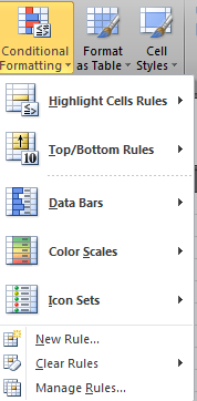
There is conditional formatting option in Excel:

You can create your own rules.
- Mark as New
- Bookmark
- Subscribe
- Mute
- Subscribe to RSS Feed
- Permalink
- Report Inappropriate Content
I know that, however, I need help with the IF() statement itself, because I am not simply comparing all cell values to a single value, but rather the product of Cell 1 - Cell 2, which will then determine what color each cell should be.
- Mark as New
- Bookmark
- Subscribe
- Mute
- Subscribe to RSS Feed
- Permalink
- Report Inappropriate Content
- Mark as New
- Bookmark
- Subscribe
- Mute
- Subscribe to RSS Feed
- Permalink
- Report Inappropriate Content
It shows you how here... I used it yesterday goodluck
https: //support.office.com/en-za/article/Use-a-formula-to-apply-conditional-formatting-in-Excel-2013-fed60dfa-1d3f-4e13-9ecb-f1951ff89d7f?ui=en-US&rs=en-ZA&ad=ZA
- Mark as New
- Bookmark
- Subscribe
- Mute
- Subscribe to RSS Feed
- Permalink
- Report Inappropriate Content
Completely agree this is a QLik community for Qik related questions. Although somebody will have the answer this is not the right place to ask
- « Previous Replies
-
- 1
- 2
- Next Replies »
