Unlock a world of possibilities! Login now and discover the exclusive benefits awaiting you.
- Qlik Community
- :
- All Forums
- :
- QlikView App Dev
- :
- Re: Format Pivot Data
- Subscribe to RSS Feed
- Mark Topic as New
- Mark Topic as Read
- Float this Topic for Current User
- Bookmark
- Subscribe
- Mute
- Printer Friendly Page
- Mark as New
- Bookmark
- Subscribe
- Mute
- Subscribe to RSS Feed
- Permalink
- Report Inappropriate Content
Format Pivot Data
I have following pivot table in my QV document
| YEAR | A | B |
| 2014 | 44,689 | 1,859,582 |
| 2015 | 43,281 | 1,931,597 |
| 2016 | 45,764 | 2,140,009 |
| 2017 | 45,399 | 2,482,854 |
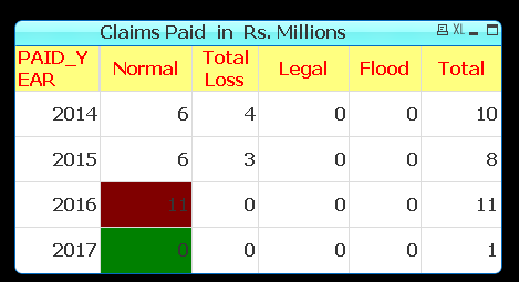
I want to highlight Max amount and Min amount in my pivot table (both font and Back ground of Cell) like given above. Pls help me
My expression is sum(amount)
Accepted Solutions
- Mark as New
- Bookmark
- Subscribe
- Mute
- Subscribe to RSS Feed
- Permalink
- Report Inappropriate Content
- Mark as New
- Bookmark
- Subscribe
- Mute
- Subscribe to RSS Feed
- Permalink
- Report Inappropriate Content
=if(Sum(Sales) = Max(Total <YEAR,Dim2> AGGR( Sum(Sales) ,YEAR,Dim2)) , red()
,if(Sum(Sales) = Min(Total <YEAR,Dim2> AGGR( Sum(Sales) ,YEAR,Dim2)) , green()) )
or
=if(Sum(Sales) = Max( AGGR(NODISTINCT Sum(Sales) ,YEAR,Dim2)) , red()
,if(Sum(Sales) = Min( AGGR(NODISTINCT Sum(Sales) ,YEAR,Dim2)) , green()) )
If a post helps to resolve your issue, please accept it as a Solution.
- Mark as New
- Bookmark
- Subscribe
- Mute
- Subscribe to RSS Feed
- Permalink
- Report Inappropriate Content
This can be done in Expression tab --> Background color & Text color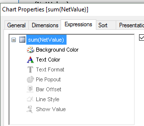
- Mark as New
- Bookmark
- Subscribe
- Mute
- Subscribe to RSS Feed
- Permalink
- Report Inappropriate Content
Thanks Vineeth
I have tried your expression. but it does not work in my Qv Doc. Pls have a look at it correct me. I am attaching my doc.
- Mark as New
- Bookmark
- Subscribe
- Mute
- Subscribe to RSS Feed
- Permalink
- Report Inappropriate Content
Check the attached
- Mark as New
- Bookmark
- Subscribe
- Mute
- Subscribe to RSS Feed
- Permalink
- Report Inappropriate Content
Hi,
try
If(RangeMin(Top(Column(1),1,NoOfRows()))=Column(1),Green(),
If(RangeMax(Top(Column(1),1,NoOfRows()))=Column(1),Red()))
Regards,
Antonio
- Mark as New
- Bookmark
- Subscribe
- Mute
- Subscribe to RSS Feed
- Permalink
- Report Inappropriate Content
Hi,
PFA fr thr application. Both text coring and background coloring is shown with example..
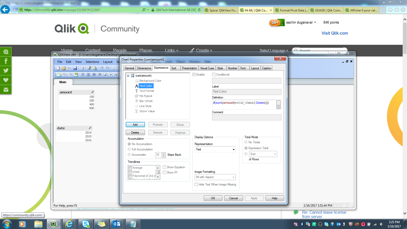
in expression tab u have to click on as shown bolow..
ANd I have created to variables in the appliactions..
please check thm out..
expression r like
vcol_Value=max(aggr(sum(amount),date))
vCol_Value2=min(aggr(sum(amount),date))
=IF(sum(amount)=vcol_Value,Red(),if(sum(amount)=vCol_Value2,Green()))
Hope it helps 