Unlock a world of possibilities! Login now and discover the exclusive benefits awaiting you.
- Qlik Community
- :
- All Forums
- :
- QlikView App Dev
- :
- Re: Pivot Table. Top3 Values
- Subscribe to RSS Feed
- Mark Topic as New
- Mark Topic as Read
- Float this Topic for Current User
- Bookmark
- Subscribe
- Mute
- Printer Friendly Page
- Mark as New
- Bookmark
- Subscribe
- Mute
- Subscribe to RSS Feed
- Permalink
- Report Inappropriate Content
Pivot Table. Top3 Values
Hi friends!
I am trying to show only 3 values per category:
- Facturas
- Recuperado
So what I tried was this: =if(aggr(rank(SUM(Datos)),[Origen Factura])<=3,[Origen Factura],Null())
But It didn´t work, it only shoy me the 3 values per one category ( facturas) due to this category is much higher/bigger than the other one but what I want is 3 values per category not 3 in total.
Many thanks
- Tags:
- pivot_table-sorting
- « Previous Replies
-
- 1
- 2
- Next Replies »
- Mark as New
- Bookmark
- Subscribe
- Mute
- Subscribe to RSS Feed
- Permalink
- Report Inappropriate Content
Hi Juan ,
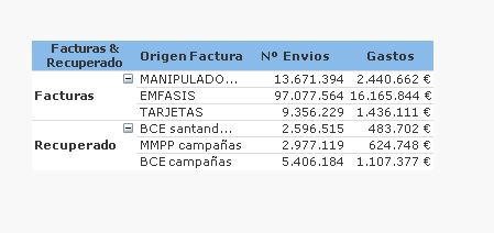
Do you want to see the result like the below pic
- Mark as New
- Bookmark
- Subscribe
- Mute
- Subscribe to RSS Feed
- Permalink
- Report Inappropriate Content
Exactly!
How do you get it?
- Mark as New
- Bookmark
- Subscribe
- Mute
- Subscribe to RSS Feed
- Permalink
- Report Inappropriate Content
Hi Juan ,
Use this expression in dimension if(aggr(rank(SUM(Datos)),[Facturas_Recuperado],[Origen Factura])<=3,[Origen Factura])
I attached qvw for your reference .
- Mark as New
- Bookmark
- Subscribe
- Mute
- Subscribe to RSS Feed
- Permalink
- Report Inappropriate Content
Expression:
=if(aggr(rank(SUM(Datos)),Facturas_Recuperado,[Origen Factura])<=3,[Origen Factura],Null())
'Supress When Value is Null' - checked.
- Mark as New
- Bookmark
- Subscribe
- Mute
- Subscribe to RSS Feed
- Permalink
- Report Inappropriate Content
create the calculated dimension as below
= aggr(if( rank(SUM(Datos),4)<=3,[Origen Factura]),Facturas_Recuperado,[Origen Factura])
check "Suppress when value is NULL"
- Mark as New
- Bookmark
- Subscribe
- Mute
- Subscribe to RSS Feed
- Permalink
- Report Inappropriate Content
does it have to be Pivot rather than Straight table?
I believe better design would be show top3 and sum of the rest as 'Others'
- Mark as New
- Bookmark
- Subscribe
- Mute
- Subscribe to RSS Feed
- Permalink
- Report Inappropriate Content
Hi,
Try this expressions
Nº Envios
=If(Rank(SUM({<Envios_Gastos={'NºENVIOS'}>}Datos)) <=3, SUM({<Envios_Gastos={'NºENVIOS'}>}Datos))
Gastos
=If(Rank(SUM({<Envios_Gastos={'GASTOS'}>}Datos)) <=3, SUM({<Envios_Gastos={'GASTOS'}>}Datos))
Regards,
Jagan.
- Mark as New
- Bookmark
- Subscribe
- Mute
- Subscribe to RSS Feed
- Permalink
- Report Inappropriate Content
The same can be done by changing your expressions like below.
Nº Envios
SUM({<[Origen Factura]= {"=aggr(rank(SUM(Datos)),Facturas_Recuperado,[Origen Factura])<=3"},Envios_Gastos={'NºENVIOS'}>}Datos)
Gastos
SUM({<[Origen Factura]= {"=aggr(rank(SUM(Datos)),Facturas_Recuperado,[Origen Factura])<=3"},Envios_Gastos={'GASTOS'}>}Datos)
- Mark as New
- Bookmark
- Subscribe
- Mute
- Subscribe to RSS Feed
- Permalink
- Report Inappropriate Content
It also works!!! Many thanks!
- « Previous Replies
-
- 1
- 2
- Next Replies »