TOP 5 in PIVOT TABLE

[MK_QSL]

I have sales table for different branches…

What I need is a pivot table with Dimensions

Branch Code

Sales Operator

Month

Expression : SUM(Sales)

I need a pivot table showing top 5 sales operator of each branch and their monthly sales achievements.

If I select Branch 01... result would be something like below...

Branch Code	Sales Operator	Month	Total	May	April	August	July	June	September
Branch 01	pshan		105,706	15,139	15,876	27,376	18,801	17,567	10,948
Branch 01	keitr		72,902	12,919	9,577	14,460	10,908	12,481	12,556
Branch 01	tferg		64,920	14,596	13,680	6,739	16,985	11,479	1,442
Branch 01	fiqba		57,937	8,505	6,771	10,878	10,780	8,714	12,289
Branch 01	antoc		42,601	8,358	6,045	7,233	9,711	6,082	5,172

[mjm]

Hello,

looking at your file I think I have achieved what you need. This is with the following sort:

Branch Code (no sorting selected)

Sales Operator (expression - sum(Sales) Descending

Month (no sorting)

This sorts according to the top sales person.

In a pivot table itself, there is no option to reduce to just show top 5. However, you could consider another chart (bar chart) where you can restrict presentation to only show 5. (Enable x axis scrollbar)

I have attached my example. I hope this helps. Please mark as answered if this helps.

[MK_QSL]

Thanks for your reply but this will not fulfill my requirements.

There should be sum RANK, AGGR and IF combination which will do my help...

[sadickbasha]

Even though you can't display only top 5 sales as there is dimension limits in Pivot table.

[israrkhan]

hope this expression will work ..

Add calculated dimension, instead of [Sales Operator]

=If(Aggr(Rank(Sum(Sales)), [Sales Operator])<=5, [Sales Operator], 'Others')

you will have 6 rows, 5 top and 1 for others.

If you dont want to show others in the pivot table, then use 'Null' like below

=If(Aggr(Rank(Sum(Sales)), [Sales Operator])<=5, [Sales Operator], 'Null')

and check suppress null value on presentation tab, you will see exactly 5 rows.

Hope it helps...

Khan

[Gysbert_Wassenaar]

See attached qvw.

[MK_QSL]

Hi Khan,

Thanks for your reply. I have done it my self by using the same by below expression... your expression is not working...

=IF(AGGR(RANK(SUM(Sales)),[Branch Code],[Sales Operator])<=5, [Sales Operator])

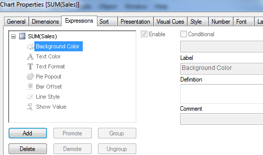
One more question.... how can I color the dimension cell ?

If May sale for particular Operator is higher in respective branch than previous month i.e. April... the background color should be Green or Red

[israrkhan]

Hi Manish,

Sure any expression will not work exactly, without seeing data model.

but meant to give an idea, and off course you have to make little changes in that, but that helped you..

for background color, put your condition here in background color, see the image

[Anonymous]

if i have a cyclic group in dimention then in that case how should i give calculated dimention?

[MK_QSL]

$(=GetCurrentField(Selection))

Use Above instead of your Dimensions below...

=IF(AGGR(RANK(SUM(Sales)),[Branch Code],[Sales Operator])<=5, [Sales Operator])