Unlock a world of possibilities! Login now and discover the exclusive benefits awaiting you.
- Qlik Community
- :
- All Forums
- :
- QlikView App Dev
- :
- Re: how to get the cumulative bucket expression of...
- Subscribe to RSS Feed
- Mark Topic as New
- Mark Topic as Read
- Float this Topic for Current User
- Bookmark
- Subscribe
- Mute
- Printer Friendly Page
- Mark as New
- Bookmark
- Subscribe
- Mute
- Subscribe to RSS Feed
- Permalink
- Report Inappropriate Content
how to get the cumulative bucket expression of a pivot to a dimension to form new pivot?
Hello,
I am working on a sales qlikview DB project. the ask is to transform the below pivot chart(chart 1 ) (note- last 3 columns are derived using expressions) in a way so that last column ('bucket') becomes the dimension and other adjacent columns gets computed (like in chart 2).
chart 1
| PARTNER_ID | Sales( PERFORMANCE) | % of Contribution to total sales | % Cumulative Contribution | Bucket- based on cumulative contirbution |
| 18915 | 1381.144578 | 17% | 17% | TOP 20% |
| 29013 | 1074.372912 | 14% | 31% | TOP 40% |
| 23580 | 938.3251691 | 12% | 43% | TOP 50% |
| 8456 | 865.3965332 | 11% | 54% | TOP 60% |
| 8760 | 707.4127103 | 9% | 63% | TOP 70% |
| 18200 | 452.48881 | 6% | 68% | TOP 70% |
| 14795 | 437.43573 | 6% | 74% | TOP 80% |
| 19142 | 433.1849702 | 5% | 79% | TOP 80% |
| 8972 | 374.08177 | 5% | 84% | TOP 90% |
| 8633 | 370.71325 | 5% | 89% | TOP 90% |
| 28683 | 201.44438 | 3% | 91% | TOP 100% |
| 5423 | 201.10581 | 3% | 94% | TOP 100% |
| 19349 | 128.40793 | 2% | 95% | TOP 100% |
| 19818 | 126.8009935 | 2% | 97% | TOP 100% |
| 8631 | 86.35097 | 1% | 98% | TOP 100% |
| 8784 | 30.31293 | 0% | 99% | TOP 100% |
Chart 2
| Percentage | # Partners | Sell thru |
| Top 10% | 0 | $0 |
| Top 20% | 1 | $1,381 |
| Top 30% | 0 | $1 |
| Top 40% | 1 | $1,074 |
| Top 50% | 1 | $938 |
| Top 60% | 1 | $865 |
| Top 70% | 2 | $1,159 |
| Top 80% | 2 | $870 |
| Top 90% | 2 | $752 |
| Top 100% | 6 | $572 |
any kind help/advice would be appreciated.
Thanks!
Avi
Accepted Solutions
- Mark as New
- Bookmark
- Subscribe
- Mute
- Subscribe to RSS Feed
- Permalink
- Report Inappropriate Content
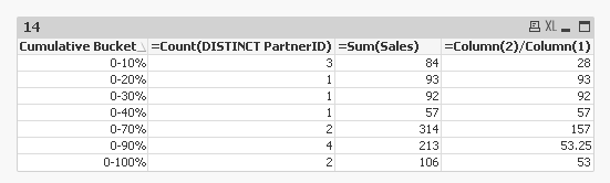
Like this?
I hope you have QV12, because you will need to use this -> The sortable Aggr function is finally here!
Dimension:
=Aggr(
If(RangeSum(Above(TOTAL Sum(Sales)/Sum(TOTAL(Sales)), 0, RowNo(TOTAL))) <= 0.10, Dual('0-10%', 1),
If(RangeSum(Above(TOTAL Sum(Sales)/Sum(TOTAL(Sales)), 0, RowNo(TOTAL))) <= 0.20, Dual('0-20%', 2),
If(RangeSum(Above(TOTAL Sum(Sales)/Sum(TOTAL(Sales)), 0, RowNo(TOTAL))) <= 0.30, Dual('0-30%', 3),
If(RangeSum(Above(TOTAL Sum(Sales)/Sum(TOTAL(Sales)), 0, RowNo(TOTAL))) <= 0.40, Dual('0-40%', 4),
If(RangeSum(Above(TOTAL Sum(Sales)/Sum(TOTAL(Sales)), 0, RowNo(TOTAL))) <= 0.50, Dual('0-50%', 5),
If(RangeSum(Above(TOTAL Sum(Sales)/Sum(TOTAL(Sales)), 0, RowNo(TOTAL))) <= 0.60, Dual('0-60%', 6),
If(RangeSum(Above(TOTAL Sum(Sales)/Sum(TOTAL(Sales)), 0, RowNo(TOTAL))) <= 0.70, Dual('0-70%', 7),
If(RangeSum(Above(TOTAL Sum(Sales)/Sum(TOTAL(Sales)), 0, RowNo(TOTAL))) <= 0.80, Dual('0-80%', 8),
If(RangeSum(Above(TOTAL Sum(Sales)/Sum(TOTAL(Sales)), 0, RowNo(TOTAL))) <= 0.90, Dual('0-90%', 9), Dual('0-100%', 10)))))))))), (PartnerID, (TEXT, ASC)))
Expressions:
1) =Count(DISTINCT PartnerID)
2) =Sum(Sales)
3) =Column(2)/Column(1)
- Mark as New
- Bookmark
- Subscribe
- Mute
- Subscribe to RSS Feed
- Permalink
- Report Inappropriate Content
Would you be able to share a sample so that we can test/play around with what you have to get you the desired output?
- Mark as New
- Bookmark
- Subscribe
- Mute
- Subscribe to RSS Feed
- Permalink
- Report Inappropriate Content
Hi Sunny,
PFA the attached QVW with sample inline load data. the chart in this QVW(chart 1) needs to be summarized like the way I have done in excel screenshot below (chart 2) based on 'cumulative bucket' column.
while I was preparing this sample chart, I came across another unusual thing- if I place the 'cumulative bucket' just next to 'cumulative %' column it does not give the correct output, but if place a column away it works fine.can you also help me understand this too(this is anyhow not important its just a curious observation ).
Chart 1

Chart 2
| cumulative bucket | Count of PartnerID | Sum of Sales | APP(column2/column1) |
| 10% | 3 | 84 | 28 |
| 100% | 2 | 106 | 53 |
| 20% | 1 | 93 | 93 |
| 30% | 1 | 92 | 92 |
| 40% | 1 | 57 | 57 |
| 70% | 2 | 314 | 157 |
| 90% | 4 | 213 | 53.25 |
| Grand Total | 14 | 959 | 68.5 |
- Mark as New
- Bookmark
- Subscribe
- Mute
- Subscribe to RSS Feed
- Permalink
- Report Inappropriate Content
Like this?
I hope you have QV12, because you will need to use this -> The sortable Aggr function is finally here!
Dimension:
=Aggr(
If(RangeSum(Above(TOTAL Sum(Sales)/Sum(TOTAL(Sales)), 0, RowNo(TOTAL))) <= 0.10, Dual('0-10%', 1),
If(RangeSum(Above(TOTAL Sum(Sales)/Sum(TOTAL(Sales)), 0, RowNo(TOTAL))) <= 0.20, Dual('0-20%', 2),
If(RangeSum(Above(TOTAL Sum(Sales)/Sum(TOTAL(Sales)), 0, RowNo(TOTAL))) <= 0.30, Dual('0-30%', 3),
If(RangeSum(Above(TOTAL Sum(Sales)/Sum(TOTAL(Sales)), 0, RowNo(TOTAL))) <= 0.40, Dual('0-40%', 4),
If(RangeSum(Above(TOTAL Sum(Sales)/Sum(TOTAL(Sales)), 0, RowNo(TOTAL))) <= 0.50, Dual('0-50%', 5),
If(RangeSum(Above(TOTAL Sum(Sales)/Sum(TOTAL(Sales)), 0, RowNo(TOTAL))) <= 0.60, Dual('0-60%', 6),
If(RangeSum(Above(TOTAL Sum(Sales)/Sum(TOTAL(Sales)), 0, RowNo(TOTAL))) <= 0.70, Dual('0-70%', 7),
If(RangeSum(Above(TOTAL Sum(Sales)/Sum(TOTAL(Sales)), 0, RowNo(TOTAL))) <= 0.80, Dual('0-80%', 8),
If(RangeSum(Above(TOTAL Sum(Sales)/Sum(TOTAL(Sales)), 0, RowNo(TOTAL))) <= 0.90, Dual('0-90%', 9), Dual('0-100%', 10)))))))))), (PartnerID, (TEXT, ASC)))
Expressions:
1) =Count(DISTINCT PartnerID)
2) =Sum(Sales)
3) =Column(2)/Column(1)
- Mark as New
- Bookmark
- Subscribe
- Mute
- Subscribe to RSS Feed
- Permalink
- Report Inappropriate Content
Thanks Sunny, it works perfectly. 
but there is one problem, when we sort the data in 'descending' sales in chart 1, then our summarized calculated dimension does not match. any suggestion on how we can alter the dimension expression to get the chart 2 as per descending sales.sorry I missed this crucial part when I first drafted.

thanks in advance for your help/suggestion.
Regards,
Avishek
- Mark as New
- Bookmark
- Subscribe
- Mute
- Subscribe to RSS Feed
- Permalink
- Report Inappropriate Content
Yes and that is because these are two different charts. You will have to decide what sorting do you want here.
- Mark as New
- Bookmark
- Subscribe
- Mute
- Subscribe to RSS Feed
- Permalink
- Report Inappropriate Content
HI Sunny,
I wanted to get the same out put but with 'sales' sorted Descending.
Thanks in advance for your kind advice/help in order to achieve this.
Avishek
- Mark as New
- Bookmark
- Subscribe
- Mute
- Subscribe to RSS Feed
- Permalink
- Report Inappropriate Content
Hello Sunny,
Were you able to tweak the expression for Chart 2? (sorted Descending SALES)
Thanks,
Avishek
- Mark as New
- Bookmark
- Subscribe
- Mute
- Subscribe to RSS Feed
- Permalink
- Report Inappropriate Content
AFAIK this cannot be done. May be someone else might be able to offer some better advice
- Mark as New
- Bookmark
- Subscribe
- Mute
- Subscribe to RSS Feed
- Permalink
- Report Inappropriate Content
Thank you Sunny, you still managed to solve it to good extent.:)
I think the requirement is little unrealistic.
let me take few more views before I give up on this.