Unlock a world of possibilities! Login now and discover the exclusive benefits awaiting you.
- Qlik Community
- :
- All Forums
- :
- QlikView
- :
- Re: Dimension label - rolling date
- Subscribe to RSS Feed
- Mark Topic as New
- Mark Topic as Read
- Float this Topic for Current User
- Bookmark
- Subscribe
- Mute
- Printer Friendly Page
- Mark as New
- Bookmark
- Subscribe
- Mute
- Subscribe to RSS Feed
- Permalink
- Report Inappropriate Content
Dimension label - rolling date
I have a field Qtr - which holds 4 values (rolling 4 quarter year). I need to display the rolling 4 quarter year as column headers (dimension labels). I've this field as a dimension in my pivot table. How to get correct result as below?
| Qtr | |||||
| 1Q 2017 | 2Q 2016 | 3Q 2016 | 4Q 2016 | 1Q 2017 | |
| 2Q 2017 | 3Q 2016 | 4Q 2016 | 1Q 2017 | 2Q 2017 | |
| 3Q 2017 | 4Q 2016 | 1Q 2017 | 2Q 2017 | 3Q 2017 | |
| 4Q 2017 | 1Q 2017 | 2Q 2017 | 3Q 2017 | 4Q 2017 |
- Tags:
- custom label
- customized columns
- dimension
- label chart
- new_to_qlik_sense
- new_to_qlikview
- rolling quarters
- rolling weeks
Accepted Solutions
- Mark as New
- Bookmark
- Subscribe
- Mute
- Subscribe to RSS Feed
- Permalink
- Report Inappropriate Content
Try this as your calculated dimension
=Pick(Dim, YR_MTH,
Ceil(Month(Max(TOTAL Date#(YR_MTH, 'YYYYMM'), 4))/3) & 'Q' & ' ' & Year(Max(TOTAL Date#(YR_MTH, 'YYYYMM'), 4)) & ' to ' & Ceil(Month(Max(TOTAL Date#(YR_MTH, 'YYYYMM'), 3))/3) & 'Q' & ' ' & Year(Max(TOTAL Date#(YR_MTH, 'YYYYMM'), 3)) & ' Change',
Ceil(Month(Max(TOTAL Date#(YR_MTH, 'YYYYMM'), 3))/3) & 'Q' & ' ' & Year(Max(TOTAL Date#(YR_MTH, 'YYYYMM'), 3)) & ' to ' & Ceil(Month(Max(TOTAL Date#(YR_MTH, 'YYYYMM'), 2))/3) & 'Q' & ' ' & Year(Max(TOTAL Date#(YR_MTH, 'YYYYMM'), 2)) & ' Change',
Ceil(Month(Max(TOTAL Date#(YR_MTH, 'YYYYMM'), 2))/3) & 'Q' & ' ' & Year(Max(TOTAL Date#(YR_MTH, 'YYYYMM'), 2)) & ' to ' & Ceil(Month(Max(TOTAL Date#(YR_MTH, 'YYYYMM'), 1))/3) & 'Q' & ' ' & Year(Max(TOTAL Date#(YR_MTH, 'YYYYMM'), 1)) & ' Change')
- Mark as New
- Bookmark
- Subscribe
- Mute
- Subscribe to RSS Feed
- Permalink
- Report Inappropriate Content
Can you explain a little more and share some sample data or a file to work on? You can drag your quarter field to top of the expression that way the quarters will become headers, is this what you are looking for?
- Mark as New
- Bookmark
- Subscribe
- Mute
- Subscribe to RSS Feed
- Permalink
- Report Inappropriate Content
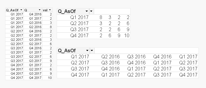
I'm not sure if you want the labels (bottom chart) or the values (top chart)
.qvw with test data and charts in the attachments
- Mark as New
- Bookmark
- Subscribe
- Mute
- Subscribe to RSS Feed
- Permalink
- Report Inappropriate Content
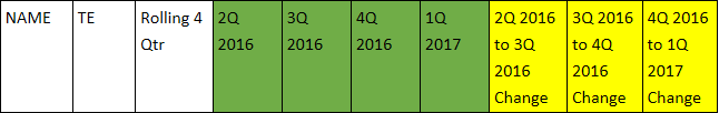
Here's what am looking for:
From the first table below, I was able to change the Header for rolling 4 quarters dynamically (green highlight)
201603 - 2Q 2016
201606 - 3Q 2016
201609 - 4Q 2016
201703 - 1Q 2017
I used this in the load script to achieve it:
RIGHT(YR_YR, 2)/3 & 'Q ' & LEFT(YR_MTH,4) AS ROLLING_4_QTR_YR

Now, I need to convert the last 3 field labels (which are hard coded value in the qlikview table above) to the right 3 columns highlighted yellow ( these quarter year value should be dynamic).
| NAME | TE | Rolling 4 Qtr | 2Q 2016 | 3Q 2016 | 4Q 2016 | 1Q 2017 | 2Q 2016 to 3Q 2016 Change | 3Q 2016 to 4Q 2016 Change | 4Q 2016 to 1Q 2017 Change |
| ABC | 1100 | 120 | 1200 | 945 | 100.00% | 0.00% | -300% | ||
| DEF | 300 | 400 | 400 | 210 | 100.00% | 0.00% | -200% |
- Mark as New
- Bookmark
- Subscribe
- Mute
- Subscribe to RSS Feed
- Permalink
- Report Inappropriate Content
Hi
Do you necessarily need the columns laid out in that way?
If not, the attached solves your problem just shown in a slightly different way
Basically I have modified slightly the load script and added a table with reference to the quarter
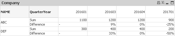
Then amended your pivot table and added an extra line which shows the % difference with the previous quarter
Hopefully it helps
Lorenzo
- Mark as New
- Bookmark
- Subscribe
- Mute
- Subscribe to RSS Feed
- Permalink
- Report Inappropriate Content
Hello All, thank you for your inputs.
I do need the table in the specified format as shown below. These are the column headers (labels). However, the quarter number and year (2Q, 3Q, 4Q, 1Q, 2016, 2017) are values that should be dynamically updated as change with quarter. I got the green part working (which is dimension) but the yellow part (which is expression in the pivot chart) doesn't work. It's hard coded right now, and this has to be dynamic instead of hard coded.
Help! please.
- Mark as New
- Bookmark
- Subscribe
- Mute
- Subscribe to RSS Feed
- Permalink
- Report Inappropriate Content
Do you always only have 4 periods you want to analyse? Will the table go from "3Q 2016" to "2Q 2017" (4 periods) or will it go "2Q 2016" to "2Q 2017" (5 periods)?
- Mark as New
- Bookmark
- Subscribe
- Mute
- Subscribe to RSS Feed
- Permalink
- Report Inappropriate Content
I always have 4 quarters to analyze. There will never be more than 4 quarters.
So, currently it is 2Q 2016, 3Q 2016, 4Q 2016, 1Q 2017
Next quarter, it'll be 3Q 2016, 4Q 2016, 1Q 2017, 2Q 2017 and
next one would be 4Q 2016, 1Q 2017, 2Q 2017, 3Q 2017
- Mark as New
- Bookmark
- Subscribe
- Mute
- Subscribe to RSS Feed
- Permalink
- Report Inappropriate Content
Try this as your calculated dimension
=Pick(Dim, YR_MTH,
Ceil(Month(Max(TOTAL Date#(YR_MTH, 'YYYYMM'), 4))/3) & 'Q' & ' ' & Year(Max(TOTAL Date#(YR_MTH, 'YYYYMM'), 4)) & ' to ' & Ceil(Month(Max(TOTAL Date#(YR_MTH, 'YYYYMM'), 3))/3) & 'Q' & ' ' & Year(Max(TOTAL Date#(YR_MTH, 'YYYYMM'), 3)) & ' Change',
Ceil(Month(Max(TOTAL Date#(YR_MTH, 'YYYYMM'), 3))/3) & 'Q' & ' ' & Year(Max(TOTAL Date#(YR_MTH, 'YYYYMM'), 3)) & ' to ' & Ceil(Month(Max(TOTAL Date#(YR_MTH, 'YYYYMM'), 2))/3) & 'Q' & ' ' & Year(Max(TOTAL Date#(YR_MTH, 'YYYYMM'), 2)) & ' Change',
Ceil(Month(Max(TOTAL Date#(YR_MTH, 'YYYYMM'), 2))/3) & 'Q' & ' ' & Year(Max(TOTAL Date#(YR_MTH, 'YYYYMM'), 2)) & ' to ' & Ceil(Month(Max(TOTAL Date#(YR_MTH, 'YYYYMM'), 1))/3) & 'Q' & ' ' & Year(Max(TOTAL Date#(YR_MTH, 'YYYYMM'), 1)) & ' Change')